Introduction
In the previous lecture, we used order parameters to distinguish order from disorder, critical exponents to describe behavior near a phase transition, and scaling laws to relate those exponents. One question, however, remained unanswered. Can we derive this behavior from a specific theory?
For example, knowing that the order parameter obeys \(m\sim(-t)^\beta\) tells us how to describe its behavior. To explain this power law, we need to understand why the system changes from favoring \(m=0\) to selecting \(m\ne0\), and why it becomes more sensitive to perturbations as the transition approaches.
The two central concepts of this lecture address two closely connected questions.
Landau theory describes the competition between states through a free energy expressed in terms of the order parameter, and predicts which state the system selects by finding its minima. In the simplest case, this free energy is a quartic polynomial. Minimizing it yields a continuous phase transition and a set of mean-field critical exponents.
The Ginzburg criterion compares fluctuations within a correlated region with the degree of order predicted by mean-field theory, testing whether an expansion about a single mean state is reliable. It is not another model of a phase transition, but a self-consistency test of the approximation just described.
The connection between them requires us to restore space to the theory. Different positions need not be in the same state, and their variations can be correlated. We will follow this reasoning step by step, from choosing the variables to testing the approximation.
Identify the order parameter → Write the free energy → Find the mean-field state → Include spatial fluctuations → Test the mean-field approximation
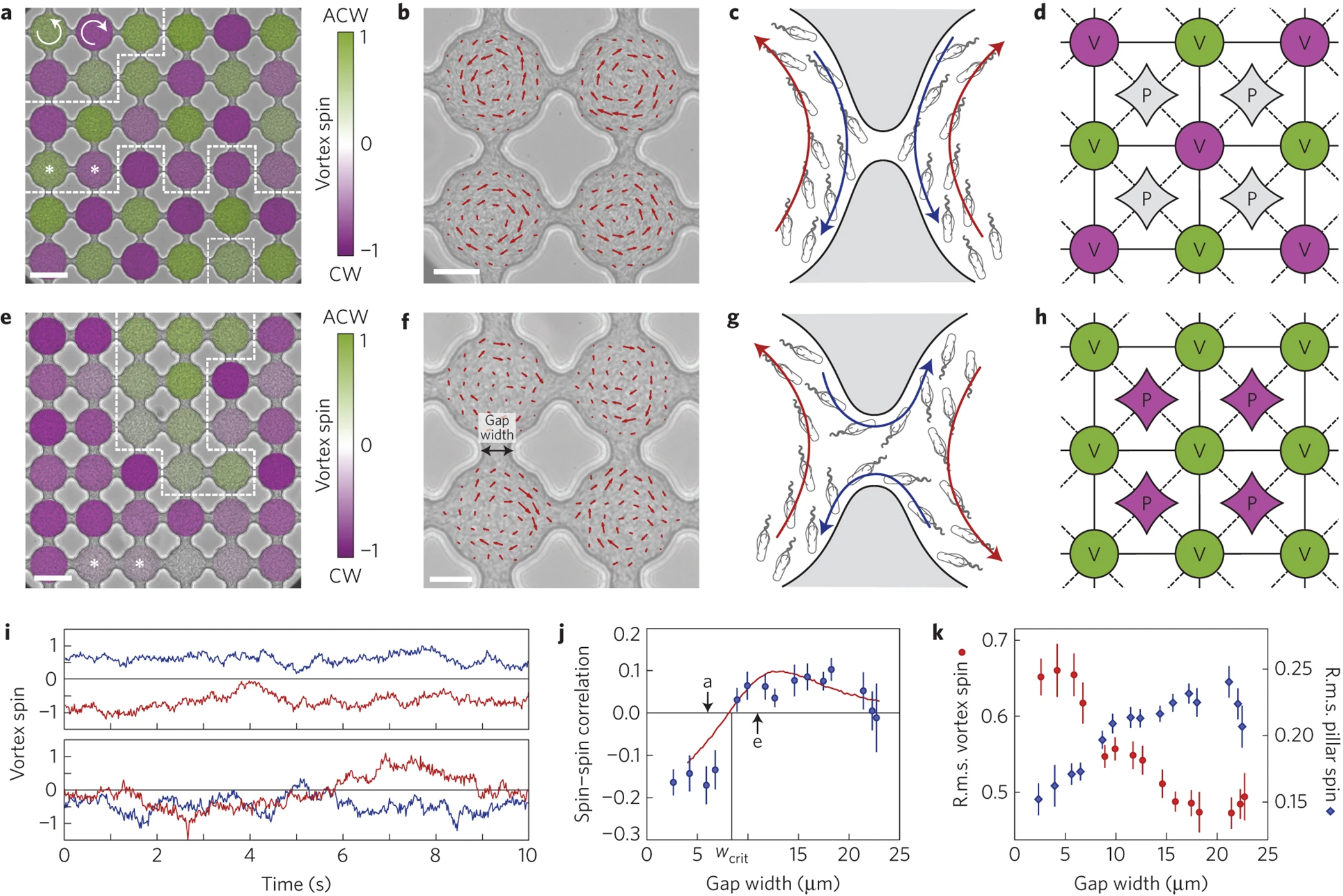
To give these concepts a concrete physical setting, we begin with an experimental study of bacterial vortex lattices. In a paper published in Nature Physics, Wioland and colleagues confined large numbers of swimming bacteria in small, interconnected circular chambers, where they formed vortices, and studied how these local rotations organized into ordered arrangements[1]. They found that changing the width of the channels between chambers could change the preference of neighboring vortices for rotating in the same or opposite directions. They explained this behavior with a model that includes interactions and fluctuations, then used a mean-field approximation to reduce it to a quartic-potential model closely related to the Landau theory developed here.
1. Order and Fluctuations in Bacterial Vortices
The significance of this experiment is that it makes the general question of how local motion gives rise to collective order directly observable and experimentally controllable. The formation of a vortex in one chamber does not determine the arrangement of the entire array[1]. Thus, collective order cannot be inferred from the properties of isolated units alone; it also depends on how those units interact. Rotation continues to fluctuate even within ordered regions. We must therefore explain not only why the system favors a particular state, but also what is neglected when we replace the actual motion with a mean state, and whether those fluctuations are large enough to compromise the predictions. The experiment itself is not an equilibrium system. Nevertheless, these two questions will lead us, respectively, to Landau theory and the Ginzburg criterion in the equilibrium reference model used in this lecture.
1.1 Why Do the Same Bacteria Form Different Rotational Arrangements?
The formation of local rotation and the ordering of an entire array are distinct problems. In these experiments, the bacterial species and basic chamber structure were held fixed, while the gaps between chambers were varied to compare the rotational relationship between neighboring vortices.
Wioland and colleagues fabricated an array of shallow circular chambers in a microfluidic device, connecting neighboring chambers by narrow channels. Under suitable confinement, the motion of many bacteria forms a collectively rotating vortex, while flow between chambers allows the vortices to influence one another[1]. The experiment first poses a very specific question. Does the vortex in one chamber prefer to rotate in the same direction as its neighbor, or in the opposite direction?
The gap between chambers is \(6\,\mu\mathrm m\). In the first half of the video, the left view shows bright-field images, while the right view adds a false-color overlay of the rotational variable. Green and purple represent opposite directions of rotation, not bacterial species or density; the second half shows the local flow field. Look for local alternating arrangements rather than a perfect checkerboard spanning the entire device. Video source: Wioland, H., Woodhouse, F. G., Dunkel, J., & Goldstein, R. E. (2016). Ferromagnetic and antiferromagnetic order in bacterial vortex lattices. Nature physics, 12(4), 341-345.
Widening the gap changes the arrangement. Locally, neighboring chambers now tend to rotate in the same direction.
Wider gaps produce regions that favor rotation in the same direction; this does not mean that all vortices maintain the same direction indefinitely. Video source: Wioland, H., Woodhouse, F. G., Dunkel, J., & Goldstein, R. E. (2016). Ferromagnetic and antiferromagnetic order in bacterial vortex lattices. Nature physics, 12(4), 341-345.
The paper calls rotation in the same direction "ferromagnetic order" and alternating rotation "antiferromagnetic order." These names describe the arrangement; they do not imply that the bacteria possess the magnetic properties invoked by the analogy. Both arrangements can be ordered. What changes is the preferred relationship between neighbors.
Order means neither immobility nor the absence of fluctuations. Local rotation strengths vary, and ordered regions can split, merge, or reverse. We need to describe both persistent statistical tendencies and departures from them. It is precisely these departures that make it necessary to test the mean-field approximation.
1.2 From a Flow Field to an Order Parameter
The videos reveal different arrangements, but a theory also needs variables that we can calculate and compare. Our immediate concern is the collective rotation within each chamber, not the motion of individual bacteria. We can therefore first compress the complex flow field in a chamber into a signed real number, then ask which average over the array can distinguish different forms of order.
Let \(V_i\) denote the rotational variable of chamber \(i\). Its sign distinguishes the two directions of rotation, and its magnitude measures the rotation strength.
The original paper obtains the flow field using particle image velocimetry and defines \(V_i\) through an angular-momentum-like spatial average within each chamber. Flow velocities are also normalized by the root-mean-square speed measured in the same experiment[1]. Thus, \(V_i\) is neither the velocity of a single bacterium nor a simple average of pixel colors. The essential physical idea is that one number describes the collective rotation of one chamber.
To study rotation in the same direction, we can average over \(N\) chambers and define
If many chambers favor the same direction, their contributions add, and \(m\) can differ appreciably from zero. If positive and negative contributions cancel, \(m\) is close to zero. A large system of moving constituents now has a collective description that can be calculated.
This average merely defines a collective observable; it does not assume that all chambers are in the same state. The mean-field approximation used in this lecture enters later, when we solve the problem by representing the states at different positions with one uniform value.
We must, however, pause to check whether this variable is appropriate. A perfectly alternating pattern of rotation can also satisfy \(m=0\), yet it is clearly not disordered. On a square lattice, assigning positive and negative weights to the two alternating sets of sites allows us to define
Here \(i_x,i_y\) are the integer lattice coordinates of a chamber. The weight cancels the alternating signs of neighboring vortices, so their contributions add with the same sign in \(m_{\mathrm{alt}}\). This is the order parameter chosen to detect an alternating arrangement.
This example makes concrete a point from Lecture 4: an order parameter must correspond to the order being studied. We cannot choose an arbitrary average and then interpret its vanishing as the absence of structure.
Uniform and alternating rotational arrangements require different order parameters. Once we have chosen the form of order to study, however, we can ask the same question in either case. How does this order emerge from a disordered background? We will first fix one ordering pattern, use its order parameter \(m\) to measure the degree of order, and investigate why the system changes from favoring \(m=0\) to favoring \(m\ne0\). Once we understand this basic process, we can return to the paper and consider competition between different arrangements.
1.3 From Describing Order to Explaining It
An order parameter tells us which state the system occupies, but not why it selects that state. Moving from description to prediction requires a comparison of the stability of states with different degrees of order. For an equilibrium system, free energy provides precisely this comparison.
Bacteria sustain their motion by continually consuming energy. We will therefore develop the method in an equilibrium reference model before returning to the experiment. The experimentally motivated ideas of a signed collective variable, interactions between neighboring regions, and fluctuations about an ordered state will connect the two descriptions.
Our reference model describes an ordinary continuous transition at finite temperature, driven by short-range interactions. The order parameter has a single real component, and \(m\) and \(-m\) are equivalent in the absence of an external field. We will see how symmetry and stability lead to a quartic polynomial in the order parameter: the simplest scalar quartic theory, usually called \(\phi^4\) theory.
Sections 2-5 will successively construct the free energy, find the mean-field state, and test the fluctuations. Section 6 will return to bacterial vortices and show how this description enters the paper's effective model.
1.4 Does the Same Average Imply the Same Arrangement?
The choice of order parameter determines which structures are retained. Comparing uniform, alternating, and disordered rotational arrangements makes the distinction clear. The ordinary average detects net rotation, but can fail to distinguish the other two, very different arrangements. Understanding this distinction tells us what \(m\) will actually describe in the free energy introduced later.
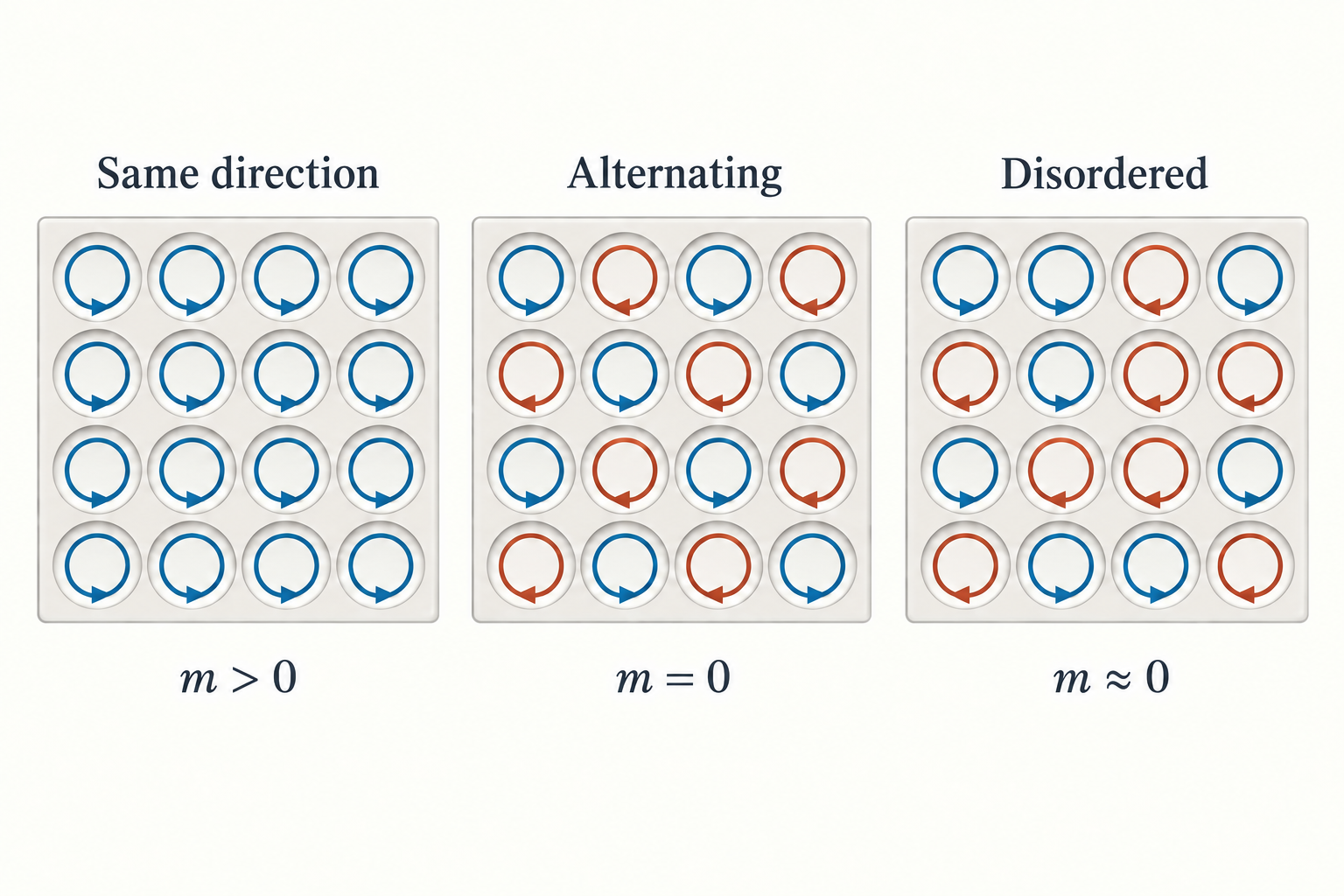
Let us calculate the averages for these arrangements explicitly. Suppose each chamber has rotation strength \(v>0\), with blue representing \(+v\) and orange representing \(-v\). All \(16\) chambers on the left are blue, so \(m=v\). The middle and right panels each contain \(8\) blue and \(8\) orange chambers. In this idealized example of equal-strength rotation, both give
The equality follows from the averaging operation itself. It adds the rotations of the chambers without recording their positions. Even if we rearrange the blue and orange chambers in the middle panel and destroy the alternating pattern, \(m\) remains unchanged as long as the numbers of the two colors stay the same. The ordinary average retains the net preference for one direction of rotation, but discards the spatial information about how those directions are distributed. Thus, \(m=0\) tells us only that positive and negative contributions cancel; it cannot, by itself, tell us whether the arrangement is ordered.
The staggered order parameter restores precisely this spatial information. Assign weights \(+1\) and \(-1\) to the two sets of checkerboard sites, choosing the positive weights to coincide with the blue sites in the middle panel. Each original \(+v\) remains unchanged, while each original \(-v\) is multiplied by \(-1\) and also becomes \(+v\). Contributions that canceled in the ordinary average now all add in the staggered average, giving \(m_{\mathrm{alt}}=v\). This calculation shows that an order parameter does more than take an average; it specifies which ordering pattern we intend to identify.
Once an ordering pattern has been chosen, we must also distinguish the sign of the order parameter from its magnitude. Reversing every vortex in the left panel changes \(m\) from \(v\) to \(-v\), but all chambers still rotate in the same direction as one another; the system has not become more disordered. Reversing an alternating arrangement likewise only exchanges the two checkerboard colors and changes the sign of \(m_{\mathrm{alt}}\). The sign distinguishes the two orientations of the same form of order; the magnitude measures the degree of that order. These are the two states meant when we later compare \(m\) and \(-m\).
We can now state the next task for Landau theory more precisely. Rather than attempting to encode every possible arrangement in one number, we first select a form of order and its order parameter, then ask whether that order can develop and how strong it becomes. In our equilibrium reference model, the positive and negative orientations should have the same free energy when no external field favors either one. Whether the system prefers a zero or a nonzero order parameter, however, remains to be calculated. The free energy \(f(m)\) introduced in the next section is the tool for comparing these different degrees of order.
2. How Landau Theory Describes Competition Between States
An order parameter distinguishes states, but does not yet explain why the system selects one of them. Landau theory supplies the missing step through the free energy, turning competition between different degrees of order into a problem that can be compared quantitatively and solved. We will first develop the idea of an effective description, then constrain the free energy by symmetry and stability, and finally identify the approximation involved in finding its minima.
2.1 Why Not Begin by Solving the Motion of Every Particle?
Solving all microscopic motion directly is not necessarily the most effective starting point for understanding a phase transition. If the order in different systems can be described by the same type of variable, it makes sense to identify their common structure first and encode material-specific differences in effective parameters. Landau's theory of phase transitions follows this approach, allowing us to construct a model without first requiring an exact solution of the microscopic problem.
Lev Davidovich Landau (1908-1968) was a Soviet theoretical physicist. In his 1937 work on phase transitions, he placed the order parameter and symmetry at the center of the theory[2]. The importance of this approach lies not in replacing a complicated curve with a polynomial, but in changing the order in which questions are asked. First identify the order that changes across the transition; then construct the simplest effective description of it.
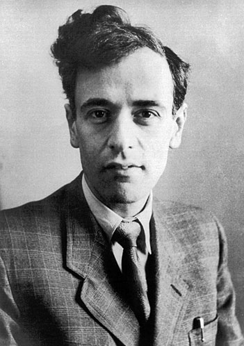
Landau and Lifshitz later gave a systematic account of this approach in Statistical Physics[3]. In 1950, Ginzburg and Landau introduced a spatially varying order parameter into the theory of superconductivity[4]. The real scalar model used in this lecture does not contain the full superconducting theory, but shares its underlying strategy. Order parameters, symmetry, and stability can constrain a theory without requiring us to solve every microscopic detail first.
Using the direction of rotation as an intuitive example, the microscopic problem could involve the position and orientation of every bacterium and the surrounding flow. A macroscopic description can instead begin by asking whether the system favors a particular collective rotation. If that is the question of interest, many microscopic details need not appear individually; they enter the coefficients of the effective description.
This compression does not guarantee that the answer is correct. It provides a tractable starting point. The power and the limitations of Landau theory must be understood as parts of the same argument.
2.2 What Does Each Term in the Polynomial Mean?
Lecture 3 showed that, at a specified temperature and under the relevant thermodynamic constraints, equilibrium is determined by the appropriate free energy. We now need to apply this principle to the order parameter, using a function to compare the cost of different degrees of order. Symmetry determines which terms are allowed, while stability determines which terms cannot be omitted. Together, these conditions lead to the quartic polynomial.
Suppose the system is constrained to have a uniform order parameter \(m\), and let \(f(m)\) denote the free-energy density of that constrained state. It answers not "Where is the system at this instant?" but "What is the free-energy cost of maintaining each possible degree of order?"
At a continuous phase transition, the order parameter emerges continuously from zero near the transition. If the coarse-grained local description admits an analytic expansion, we can organize it in powers of \(m\). Equivalence of the two orientations at zero external field requires
Odd powers such as \(m\) and \(m^3\) therefore cannot appear on their own. Retaining the lowest-order terms needed to describe an ordinary continuous transition gives
This is the Landau free energy used in this lecture, with \(u>0\). Its terms play distinct roles in the competition between states.
- \(f_0\) is a regular background independent of \(m\); it does not affect the locations of the minima.
- \(r\) determines the curvature near the origin. For \(r>0\), a small nonzero \(m\) raises the free energy; for \(r<0\), moving away from zero lowers it.
- \(u>0\) provides the lowest-order stabilizing contribution. When \(r<0\) favors nonzero order, the quartic term prevents \(m\) from growing without bound.
- \(h\) is the external field conjugate to \(m\). Through \(-hm\), it favors one orientation and removes the equivalence of the two otherwise symmetric states.
An "external field" need not be a magnetic field. Here it means a control variable that couples linearly to the order parameter in the free energy. For a rotational variable, we can think of a bias that selects one handedness of rotation. This does not imply that the paper applied or calibrated such an experimental control.
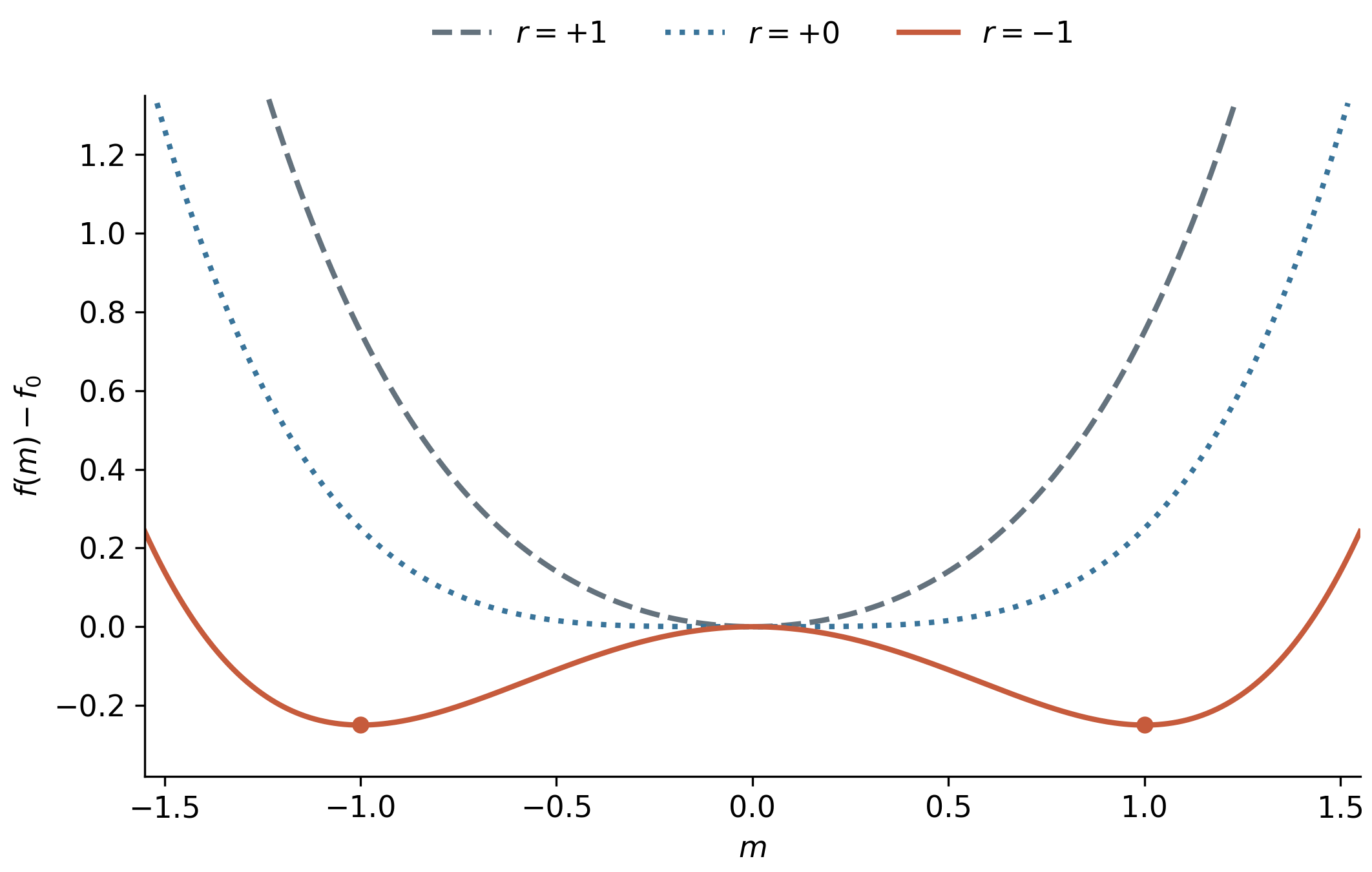
The important point is not to memorize three curves, but to understand the competition between the quadratic and quartic terms. The quadratic term determines whether order is favored; the quartic term determines where its growth stops. When the quadratic coefficient changes sign, the minima can move continuously away from the origin to either side.
What we are expanding is an effective local free energy that retains the order parameter, not the exact thermodynamic free energy obtained after all long-wavelength fluctuations have been accounted for. A smooth local polynomial can therefore serve as the starting point even though the final equilibrium free energy becomes nonanalytic at the transition.
2.3 What Approximation Is Made When We Minimize the Free Energy?
Having written down the free energy, we must explain how it determines equilibrium. Finding its minima is not an additional rule imposed on the theory; it follows from comparing the statistical weights of different states. The crucial restriction is that we initially compare only spatially uniform configurations. This makes the problem tractable, but leaves out spatial fluctuations that we will later need to examine.
In the equilibrium reference model, the statistical weight of a uniform state is proportional to
Here \(\mathcal V\) is the system volume, \(T\) the absolute temperature, and \(k_B\) Boltzmann's constant. We avoid using \(V\) for volume to distinguish it from the chamber rotation variables \(V_i\). For a large volume, even a small difference in free-energy density produces a large difference in statistical weight. Consequently, in a calculation restricted to uniform states, the minima dominate the equilibrium result.
Set \(h=0\) first. The stationarity condition is
This gives \(m=0\) and two nonzero solutions that exist only for \(r<0\). Their stability is determined by the second derivative,
For \(r>0\), the curvature at \(m=0\) is positive, so this is a stable minimum. For \(r<0\), the curvature at the origin is negative, making it an unstable maximum. The new stable solutions are
The two signs represent two equivalent ordered branches. The free energy favors neither orientation, yet a macroscopic ordered phase can select one of them. This is spontaneous symmetry breaking. In a finite system observed for sufficiently long times, reversals between the two orientations can restore a vanishing overall average. A nonzero spontaneous order parameter therefore refers to a selected ordered branch, or is defined by taking the zero-field limit after the thermodynamic limit.
We can now identify precisely where the mean-field approximation enters. We represent the equilibrium background by one uniform value \(m_0\) and determine it from the equation for a free-energy minimum, without yet calculating the feedback of spatial fluctuations on that equation. We have not tested whether the actual system remains close to this background everywhere.
Landau theory and the mean-field approximation are therefore related, but not synonymous. The former specifies the form of an effective free energy; the latter is one approximation for solving it. Even within the same quartic theory, a proper treatment of fluctuations can yield critical behavior different from that predicted by the uniform minimum.
3. From Mean-Field Predictions to Critical Behavior
Once the stable minima are known, the geometry of the free energy can be translated into observable behavior. The location of a minimum determines the order parameter, its local curvature determines the response to an external field, and the free energy along the equilibrium branch determines the entropy and specific heat. Comparing these results with the definitions in the previous lecture shows how critical exponents can be derived from a single theory.
3.1 Why Does the Order Parameter Emerge with a Square-Root Dependence?
The movement of the minima away from the origin indicates the onset of order, but does not yet tell us how rapidly that order develops. To obtain a critical exponent, we must relate changes in the free-energy coefficients to the distance from criticality and identify the leading power in the stable solution. This turns the continuous bifurcation seen in the figure into the square-root law for the order parameter.
The previous lecture introduced the reduced temperature as a measure of relative distance from the critical point. Working for now within uniform mean-field theory, let \(r\) change sign at a temperature \(T_0\), and write
\(T_0\) is the critical temperature predicted by this approximation. We retain the subscript because fluctuations may shift the true critical temperature. The coefficient \(a\) gives the slope of the quadratic coefficient near criticality; for now, we replace the smoothly varying \(u\) by its positive value near the transition.
Substituting into the minimum found above gives, on the selected positive ordered branch,
Comparison with the definition \(m_0\sim(-t_0)^\beta\) yields
This exponent has not been assumed independently. It follows from the balance between \(|r|m\) and \(um^3\) in the equation for the minimum. Equating their magnitudes gives \(m^2\sim |r|/u\). For the first time, we have calculated a critical exponent from the structure of the free energy.
We are calculating the collective order parameter of an idealized equilibrium model. The appearance of stable rotation in a single chamber does not, by itself, constitute a continuous thermodynamic phase transition. Bistability of one variable and a collective phase transition involving infinitely many degrees of freedom must remain distinct.
3.2 Why Does a Flatter Potential Well Produce a Larger Response?
Knowing the location of a minimum is not enough. Two stable states can differ substantially in their sensitivity to perturbations. To describe this difference, we examine how a weak external field shifts the minimum and relate the size of that shift to the curvature of the potential well. The enhanced response will then become a quantitative prediction.
Restoring a small external field \(h\) changes the condition for a minimum to
This is the equation of state relating the external bias to the degree of order. Define the linear susceptibility as \(\chi=\partial m/\partial h\). Differentiating the equation of state at fixed temperature gives
On a stable zero-field branch, define
and obtain
\(\kappa\) is the curvature near the minimum, and thus measures the restoring strength against a departure from that state. A large curvature makes a departure costly; a small curvature allows the same external field to shift the equilibrium value much farther. In the free-energy picture, a divergent response means that the potential becomes increasingly flat near the stable state.
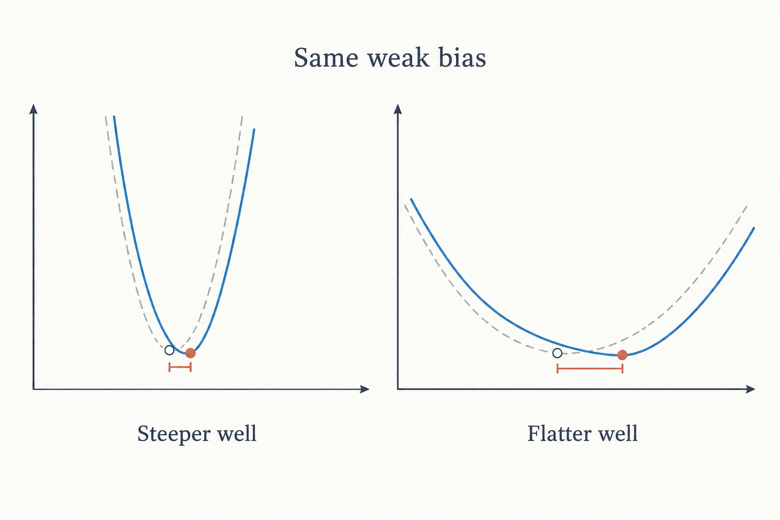
On the disordered side, \(m_0=0\), so \(\kappa_+=r\). On the ordered side, \(m_0^2=-r/u\), so \(\kappa_-=2|r|\). Therefore,
Both sides give \(\gamma_{\mathrm{MF}}=1\), but with different amplitudes. At \(r=0\), the equation of state reduces to \(h=um^3\), yielding the critical-isotherm exponent \(\delta_{\mathrm{MF}}=3\). All three exponents follow from the same equation for the minimum, rather than from three unrelated empirical laws.
3.3 Why Is It Still a Phase Transition if There Is No Latent Heat?
The order parameter and susceptibility reveal changes in the ordered state, but a thermodynamic phase transition must also be identified in the equilibrium free energy. The ordinary continuous transition considered here has no finite entropy jump, yet higher derivatives of the free energy can still be discontinuous. Substituting the stable solution into the original polynomial shows how a specific-heat anomaly arises without latent heat.
Substituting the stable solution into the free energy and subtracting the regular background gives
On the disordered side, the minimum remains at the origin. On the ordered side, selecting nonzero \(m_0\) produces a finite reduction in free energy. The two branches have the same value and first temperature derivative at \(t_0=0\), but different second derivatives.
The thermodynamic relations from Lecture 3 now clarify the classification of phase transitions discussed in Lecture 4. The entropy density is \(s=-\partial f_{\mathrm{eq}}/\partial T\), and the specific-heat density is \(C=-T\partial^2f_{\mathrm{eq}}/\partial T^2\). Here the entropy has no finite jump, so there is no latent heat. The ordering contribution to the specific heat nevertheless has a finite jump, corresponding to \(\alpha_{\mathrm{MF}}=0\). This does not mean that the total specific heat vanishes, nor does \(\alpha=0\) necessarily imply a logarithmic divergence. The actual form must be determined by calculation.
A brief comparison with latent heat is useful here. At a reversible transition under constant pressure, two phases of the same amount of material satisfy \(\Delta G=0\) at coexistence. Consequently,
Here \(G\) is the Gibbs free energy, \(T_{\mathrm{tr}}\) the transition temperature, and \(L\) the latent heat absorbed. If a pure ice-water mixture at standard atmospheric pressure is heated slowly, the supplied heat can change the proportions of the two phases without appreciably raising the temperature, as long as some ice remains. Adding heat need not raise the temperature, because energy can instead change how matter is organized. The continuous transition in this section has no such finite entropy jump, but singular behavior can still appear in higher derivatives.
A constant-temperature heating plateau is therefore not the sole test for a phase transition. A first-order transition requires a discontinuity in a first derivative of the appropriate free energy, but that derivative need not be the entropy, so latent heat need not accompany it. The essential point here is that both our calculated free energy and its first temperature derivative are continuous; the anomaly appears in higher derivatives.
The mean-field prediction is now quite complete. A closer look at the derivation, however, reveals that it has made almost no use of spatial dimension. This is not because dimension is unimportant, but because we have not yet allowed different positions to behave differently. We must now restore that freedom.
4. Spatial Fluctuations and the Correlation Length
The preceding calculation compressed the entire system into one uniform order parameter. It could describe a collective preference, but not differences between regions. We now restore spatial dependence so that local departures and their mutual influence enter the free energy. The cost of variations between neighboring regions, together with the local restoring strength, determines the correlation length and provides a basis for estimating the size of fluctuations.
4.1 The Missing Cost of Variation Between Neighboring Regions
Returning to the videos, the array does not always occupy a single uniform rotational state. One region may favor one direction, while another behaves differently. Retaining these structures requires both a position-dependent order parameter and interactions between neighboring regions. Simply assigning the same local potential to every position cannot explain spatial coordination.
We therefore generalize the uniform order parameter to \(m(\mathbf x)\), where \(\mathbf x\) denotes position and \(m(\mathbf x)\) measures the degree of order in a small surrounding region. This is the basic idea of coarse-graining introduced in Lecture 1: reduce microscopic detail while retaining spatial structures that still matter. Coarse-graining does not mean replacing the entire system with a constant.
Assigning the same local potential to each position is not sufficient. If neighboring regions could independently choose positive or negative orientations at no cost, there would be no reason for an extended region of uniformly oriented order to form. An interaction that favors similar values of neighboring variables must impose a cost on spatial variation.
On a discrete lattice, this can be seen directly from a single interaction bond. For \(J>0\),
The last two terms can be absorbed into the local quadratic coefficient. The first explicitly penalizes differences between neighboring positions. When variations are sufficiently slow, finite differences can be replaced by spatial derivatives, giving the Landau-Ginzburg free-energy functional
A "functional" takes an entire spatial distribution as its input rather than a single number; its output is still a free energy. The integral adds the contributions from all positions, and \(f(m)\) is the local quartic free energy of Section 2. The coefficient \(c>0\) measures the cost of spatial variation, \(d\) is the spatial dimension, and \(\nabla m\) measures how rapidly the field varies in space. A background term independent of \(m\) does not affect the variations or fluctuations considered below and can be omitted.
The roles of the two contributions are now clear. The local potential determines the preferred value at each position; the gradient term determines how neighboring positions coordinate. For an alternating arrangement, the field suitable for a smooth description is the order-parameter field with the alternating signs removed, not the original alternating variable treated as though it varied slowly.
4.2 The Correlation Length Comes from Competing Costs
The gradient term allows a local change to influence neighboring regions, but that influence need not remain equally strong at all distances. The local potential tends to restore each region to its stable value, while spatial coupling favors coordinated changes at neighboring positions. Comparing these effects gives a characteristic decay length and explains why it grows near the critical point.
Choose a stable background \(m_0\) and write the actual field as
Here \(\delta m\) is the departure from the background. Because \(m_0\) already satisfies the equation for the minimum, the linear term vanishes. Retaining only quadratic terms gives
The curvature \(\kappa\) is the same quantity introduced in the preceding section. The first term resists departures from the local stable value; the second resists rapid spatial changes in those departures. Retaining only quadratic terms is called the Gaussian approximation, because the corresponding statistical weight for fluctuations is Gaussian.
Suppose a departure changes appreciably over a length \(L\). Its gradient is of order \(\delta m/L\), so the relative importance of the two terms is set by \(\kappa\) and \(c/L^2\). The length at which they become comparable is
This is the correlation length in the present Gaussian theory. It is not an arbitrarily drawn domain diameter, but the characteristic scale set by competition between local restoration and spatial coordination. The same length appears in the equilibrium equation for a small perturbation. Along one spatial direction, away from the source of the perturbation,
The decaying solution is \(\delta m\propto e^{-x/\xi}\). In this equilibrium Gaussian model, the fluctuation-response relation connects the static response to the connected correlations of spontaneous fluctuations; both have the same decay length. The response length is therefore also the correlation length. In higher dimensions, the correlation function includes additional geometric factors, but away from criticality its long-distance decay is still controlled by this \(\xi\).
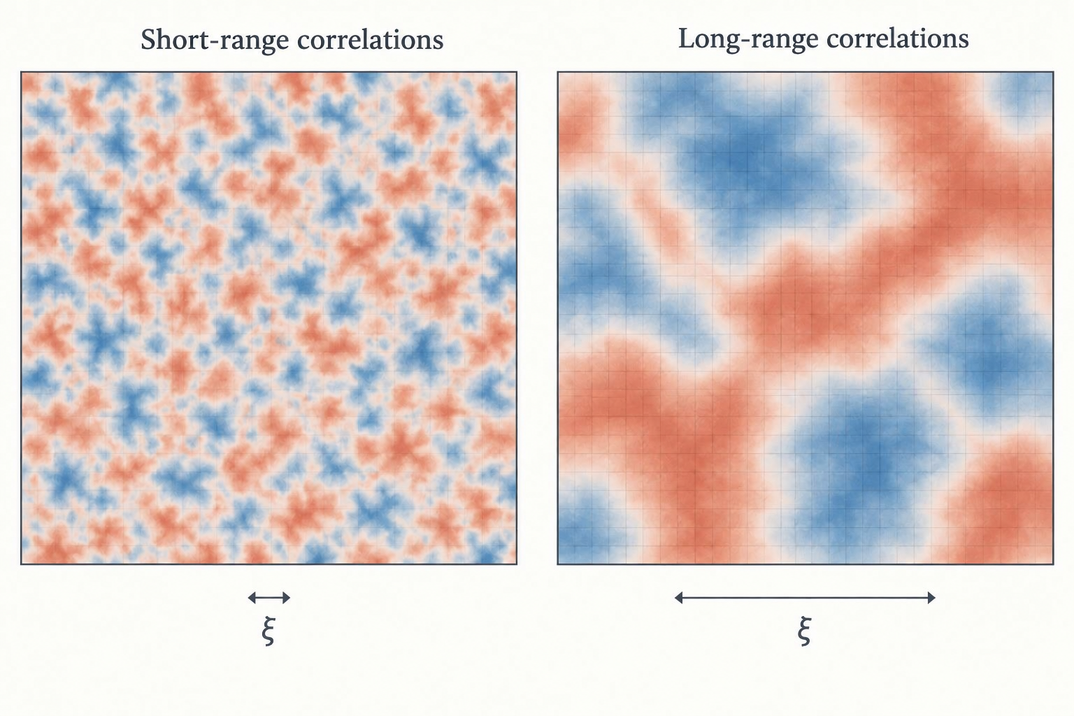
A flatter potential well therefore does two things. It allows a weak external field to produce a large response, and it allows a local departure to influence more distant positions. In the present approximation, the same curvature connects the two effects through
These are Gaussian results for this model, not unconditional identities for all systems. Since the mean-field curvature obeys \(\kappa\propto|t_0|\), we have \(\xi\propto|t_0|^{-1/2}\) and hence \(\nu_{\mathrm{MF}}=1/2\). The susceptibility and correlation length, defined independently in the previous lecture, now have a common physical origin.
4.3 Why Must We Still Test the Gaussian Fluctuations?
The correlation length tells us how far fluctuations extend, but not whether their amplitude is sufficiently small. A Gaussian calculation retains only quadratic terms and presupposes that higher-order terms provide small corrections. To test that assumption, we must estimate how far the average within a correlated region departs from the background, then compare that departure with the ordered background itself.
Consider a region with side length of order \(\xi\), and denote the spatial average of the field within it by \(\overline m_\xi\). In the selected ordered phase, its statistical mean is \(m_0\), but its value still varies between configurations. We define the variance of this variation by
The angle brackets denote a statistical average over many possible configurations, not another spatial average of the same image.
Why choose \(\xi\) rather than the size of the whole sample? A large sample can contain many correlated regions. Its overall average may remain stable even when fluctuations within each region are substantial. A stable macroscopic average does not imply that correlations within regions can be neglected. Testing a critical theory requires us to examine the correlation scale that governs critical behavior.
At the scale \(\xi\), the local quadratic term and the gradient term are of the same order. Consequently, a departure \(\delta\overline m_\xi\) of the regional average from the background has a free-energy cost of order
Here \(\xi^d\) is the correlation volume. Insert this quadratic cost into the equilibrium weight \(e^{-\Delta F_\xi/(k_BT)}\) and compare it with the standard Gaussian form \(e^{-x^2/(2\sigma^2)}\). A larger quadratic coefficient gives a narrower distribution and a smaller variance. The coefficient here is of order \(\kappa\xi^d/(k_BT)\), so
The symbol \(\sim\) indicates that finite constants depending on the shape of the region and the averaging procedure have been omitted. This result applies when the correlation length is much larger than the coarse-graining scale. Our concern is how it varies with \(\kappa\) and \(\xi\), rather than the exact coefficient for a particular window shape.
This estimate does not treat the region as a collection of independent particles. If we divide it into \(n\) equal-volume coarse-grained cells and denote each cell's departure from the background by \(\delta m_i\), the variance of the regional average is, by definition,
In addition to each cell's own variance, this sum retains cross-correlations between different cells. The \(i\ne j\) terms can simply be discarded only when the cells are independent. We chose a correlated region precisely because the variations within it cannot be treated as fully independent. The free-energy estimate above retains this coordination through the gradient term and then evaluates fluctuations of the regional average. It therefore avoids simply inserting the number of microscopic particles into a formula for independent samples.
We now have both quantities needed for the comparison: the background \(m_0\) and the typical departure \(\sigma_\xi\). The next step introduces no new model. It tests whether the approximation just made is self-consistent.
5. The Ginzburg Criterion and the Domain of Validity of Mean-Field Theory
We now have two results: the ordered background predicted by mean-field theory, and the fluctuations within a correlated region calculated about that background. The Ginzburg criterion compares them on the same scale, using the size of the neglected contribution to test the original approximation. This comparison will also explain why dimension matters and how wide the critical region of mean-field failure is.
5.1 Relative Fluctuations Determine Self-Consistency
The existence of fluctuations at finite temperature is not, by itself, a reason to reject the mean-field approximation. The relevant question is whether typical fluctuations are small relative to the background used as the zeroth-order solution. This comparison has a direct physical interpretation and can also be understood from the relative sizes of higher-order terms in the free-energy expansion.
If \(\sigma_\xi\ll |m_0|\), the average within a correlated region usually deviates only slightly from the background. Using that background as the zeroth-order solution is then a reasonable starting point.
If \(\sigma_\xi\) is already of the same order as \(|m_0|\), the variations can no longer be called "small departures." The uniform minimum can still be written down, but the approximation that justified its use has lost its basis. We define a dimensionless ratio of the variance to the squared background and require
This is the essential content of the Ginzburg criterion[5]. The numerator measures the neglected fluctuations within a correlated region; the denominator measures the ordered background retained in the approximation. Their comparison determines whether an expansion starting from mean-field theory is self-consistent.
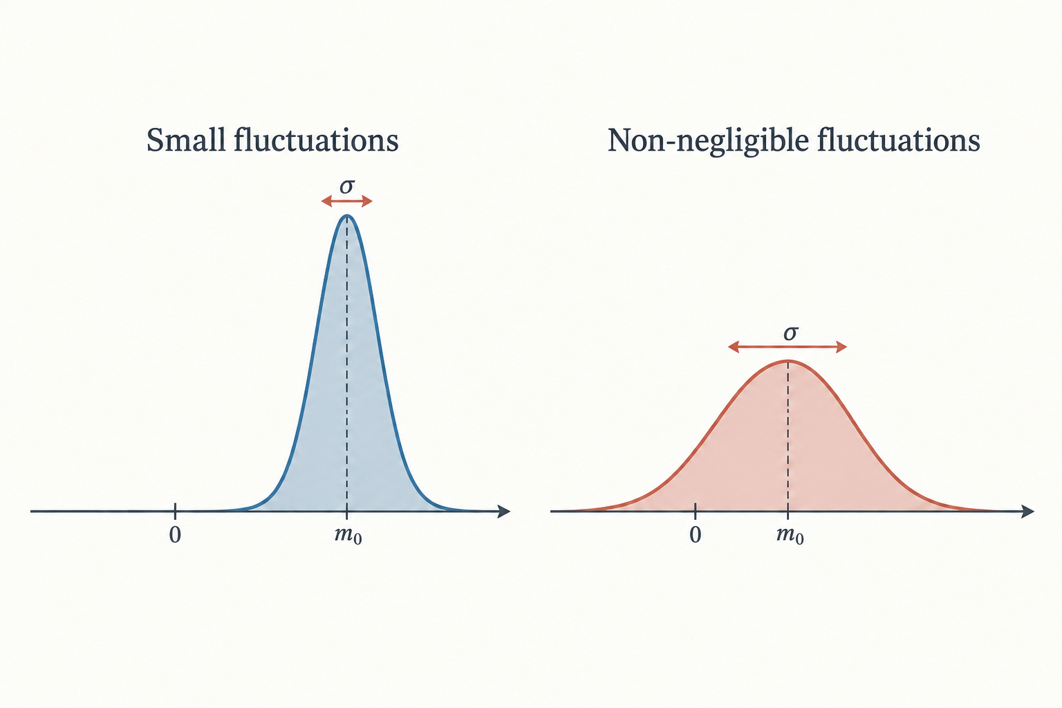
The polynomial itself explains why the background is the appropriate reference. At an ordered minimum, \(\kappa=2u m_0^2\). In an expansion about that minimum, the cubic term relative to the quadratic term is of order \(\delta m/m_0\), while the quartic term is controlled by the square of this ratio. When typical departures approach the size of the background, the neglected nonlinear terms are therefore no longer small corrections.
We will estimate this ratio from the ordered side, where a nonzero \(m_0\) provides a reference for comparison. A corresponding test also exists on the disordered side, but we cannot divide by a zero background. There, self-consistency must instead be assessed through fluctuation corrections to quantities such as the susceptibility.
5.2 Why Does Four Dimensions Emerge Naturally?
The criterion tells us what to compare, but we still need to determine how the ratio changes with distance from criticality. The background, restoring strength, and correlation volume all vary, and the growth of the correlation volume depends directly on spatial dimension. Combining these changes reveals four dimensions as the boundary between different scaling behaviors, rather than merely a number to memorize.
Before calculating, we must distinguish a shift in the location of the critical point, because fluctuations can move the critical temperature. We now absorb the regular shift of the critical point into the parameter definitions and use
to measure distance from the actual critical point. Within the self-consistent mean-field regime, the leading estimates still take the form \(m_0^2\sim a|t|/u\) and \(\kappa\sim a|t|\), with \(a\) now allowed to include a finite redefinition of the parameters. A shift in the critical point and a change in critical exponents are different effects. We are testing the singular fluctuations relevant to the latter, rather than mistaking a shift in critical temperature for a failure of the approximation.
Substituting the variance estimate from Section 4 into the criterion gives
Using \(\kappa\sim a|t|\) and \(\xi\sim\sqrt{c/(a|t|)}\) then yields
This expression can be read step by step. The squared background decreases as \(|t|\), and the restoring strength also decreases as \(|t|\), while the correlation volume grows as \(|t|^{-d/2}\). Only when all three changes are combined does the exponent \((d-4)/2\) emerge. Dimension is not a label attached afterward; it enters through the size of the region whose fluctuations are correlated.
Writing the finite prefactor as \(\overline g_0\), we can express the result more compactly as
\(\overline g_0\) is a dimensionless prefactor measuring fluctuation strength. It depends on microscopic parameters, normalization, and the chosen averaging window; it is not a constant shared by all materials. For example, choosing the reference length \(\xi_0=\sqrt{c/a}\) gives \(\overline g_0\sim k_BT_c/(a^2\xi_0^d/u)\). The quantity \(a^2/u\) has units of free-energy density and becomes an energy only after multiplication by the volume \(\xi_0^d\). The ratio is therefore indeed dimensionless.
Comparing dimensions reveals three different trends near criticality.
- For \(d<4\), provided a finite-temperature continuous transition exists, long-wavelength relative fluctuations grow as the critical point is approached, and mean-field theory eventually loses self-consistency. If the system has no such transition, this conclusion cannot be interpreted as merely requiring corrections to a few exponents.
- For \(d>4\), singular long-wavelength corrections become relatively weaker, and the leading critical exponents of an ordinary continuous transition can take their mean-field values. This does not mean that all short-distance corrections vanish.
- For \(d=4\), simple power counting predicts neither growth nor decay. Logarithmic corrections must be examined before fluctuations can be declared irrelevant.
The upper critical dimension of this short-range scalar quartic theory is therefore \(d_c=4\). "Four dimensions" here denotes a theoretical boundary between dimensional regimes. It does not mean that the bacterial experiment takes place in four dimensions, or that every phase transition has the same upper critical dimension.
5.3 How Wide Is the Ginzburg Region?
For systems below four dimensions that support a finite-temperature continuous transition, relative fluctuations grow as criticality is approached. How close one must get before they become important also depends on the model parameters. The Ginzburg number turns this question into an estimate of a critical temperature range. It explains why mean-field theory can work over an interval yet become unreliable closer to the critical point.
For \(d<4\), setting \(\mathcal R_G\) to order \(1\) gives the Ginzburg number
It estimates the width of the critical temperature region where mean-field theory begins to lose self-consistency. If \(\mathrm{Gi}\ll1\), there may be a window
The left inequality keeps fluctuations small; the right keeps us close enough to criticality for the low-order Landau expansion to remain appropriate. There is therefore no contradiction between saying that mean-field theory is useful and that it fails near the critical point. Experiments may display mean-field-like behavior over a substantial interval, with clear departures appearing only inside a narrower critical region.
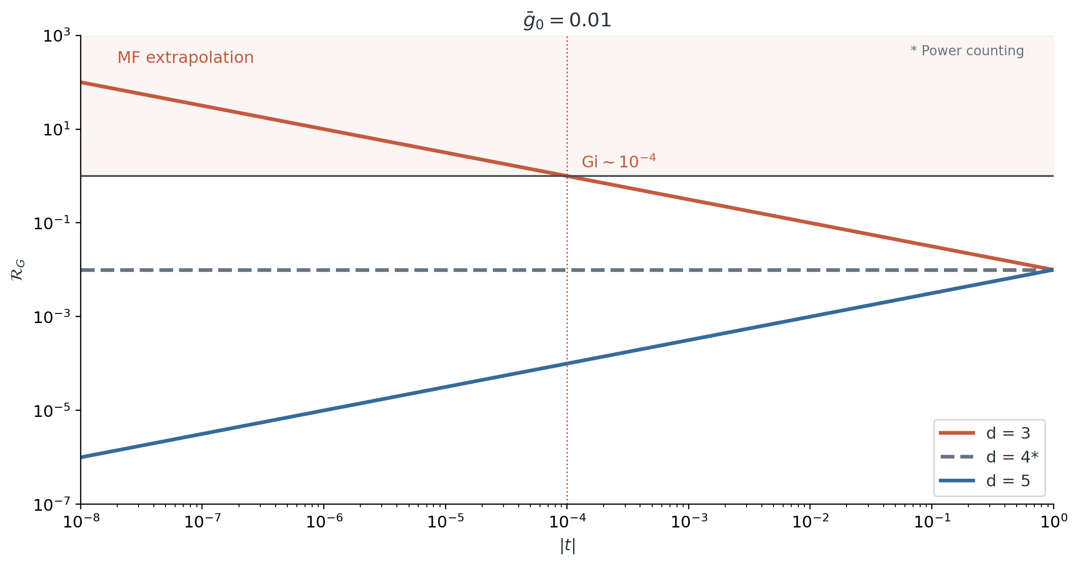
For example, take three dimensions and again set \(\overline g_0=0.01\). At \(|t|=10^{-2}\), \(\mathcal R_G\simeq0.1\); by \(|t|=10^{-4}\), it reaches \(1\). This compares magnitudes within the same approximation; it is not an estimate of a Ginzburg number from an experimental image. Moreover, \(\mathrm{Gi}\) is a crossover scale, not a new thermodynamic phase boundary.
A further point deserves attention. Increasing relative fluctuations do not require every absolute fluctuation measure to diverge. In three dimensions, the present Gaussian estimate gives
As \(\xi\) grows, the region over which we average also grows. The absolute variance of the regional average can therefore decrease, while the squared background decreases faster and their ratio increases. What fails is the condition that the background be much larger than its own fluctuations.
5.4 The Criterion Defines a Boundary; the Renormalization Group Explains What Lies Beyond
Establishing that mean-field theory fails is not the same as calculating the correct critical behavior. Landau theory provides a tractable starting point, and the Ginzburg criterion specifies when that starting point is valid. When its conditions no longer hold, we need a way to reorganize the calculation of fluctuations. This unresolved problem leads us to the renormalization group.
The criterion itself does not supply new values of \(\beta\) or \(\nu\). Once \(\mathcal R_G\) is no longer small, adding a single large correction is not reliable, because subsequent corrections may be equally important. We must instead reorganize the calculation, treating fluctuations at different scales successively while updating the interactions among the remaining variables.
This returns us to the question raised in Lecture 2 of why effective parameters must change with the observation scale. It is not because we wish to relabel the same system, but because eliminating fluctuations changes the effective description of what remains. The Ginzburg criterion identifies the limits of mean-field theory; the renormalization group provides a way to go beyond them.
6. Understanding Bacterial Vortices with a Quartic Model
With free energy, interactions, and fluctuations now distinguished, we can return to the opening paper without having to master every experimental and computational detail at once. We will first identify how channel geometry changes the interactions between vortices, then examine the connection between the authors' effective model and the equilibrium theory developed here, and finally use a small calculation to illustrate the basic mechanism. Throughout, we will distinguish experimental observations, model approximations, and the teaching demonstration.

6.1 How Channel Geometry Changes the Effective Interaction
The key difference between the two opening videos is that the preferred arrangement of neighboring vortices changes with the gap width. The paper traces this change to motion near the boundaries, then constructs effective interactions using both chamber and pillar variables. Following this mechanism explains why changing channel geometry alone can change the resulting ordered arrangement.
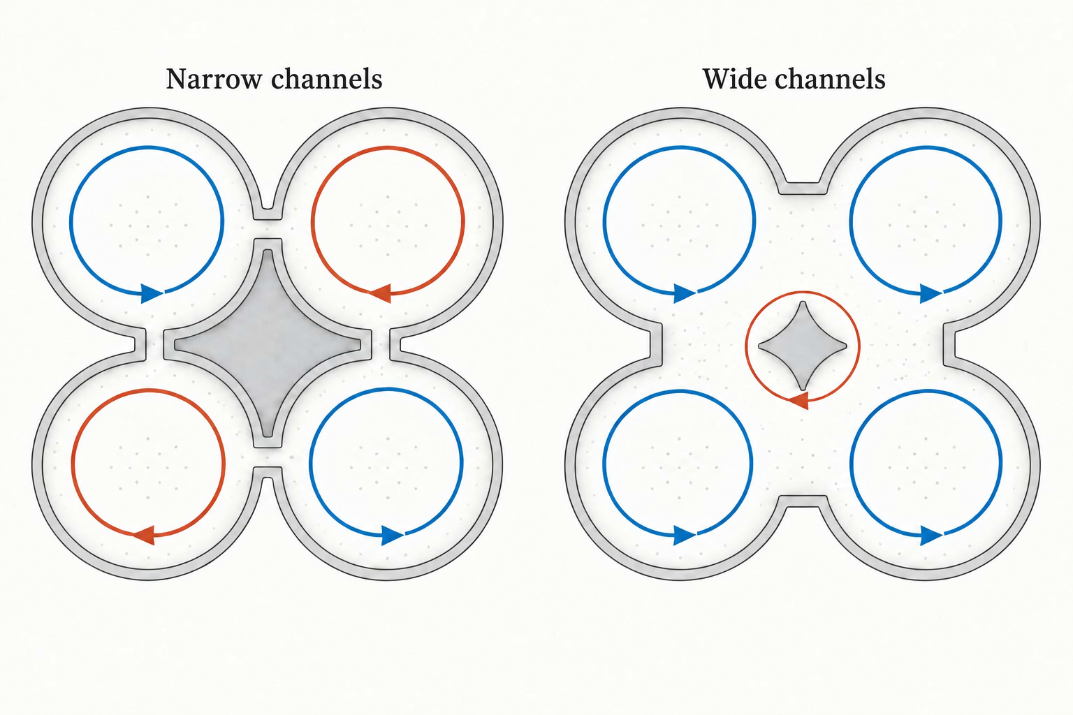
The experiments found different mean nearest-neighbor rotational correlations on either side of a gap width of approximately \(8\,\mu\mathrm m\) in the square lattice. At larger gaps, approaching approximately \(20\,\mu\mathrm m\) and beyond, individual chambers gradually cease to confine stable vortices. These two changes must not be conflated. The first concerns the preferred relationship between neighboring rotations; the second concerns whether the local vortex itself can persist[1]. Another distinction matters when reading the paper: it uses \(\chi\) for the normalized nearest-neighbor correlation, whereas Section 3 of this lecture uses \(\chi\) for the response to an external field. They are not the same observable.
The mechanism hinges on motion near the chamber boundaries. In addition to collective flow within the chambers, bacteria form streams along the boundaries. At narrow gaps, these boundary streams remain largely around their respective chambers, and the interaction between neighboring chambers favors opposite collective rotations. When the gaps widen, the paths of the boundary streams change. They can circulate around the star-shaped pillars between chambers, causing chambers surrounding the same pillar to favor rotation in the same direction[1].
The authors' full model therefore includes not only chamber rotations \(V_i\), but also circulations \(P_j\) around the pillars. This is not an attempt to make the equations more complicated. Rather, the motion capable of reversing the effective interaction cannot be omitted at the outset. The two sets of variables together define the model. Its parameters are estimated from time series of the experimental flow field, and the model is then tested against the observed trends in nearest-neighbor correlations.
The paper then approximately eliminates the pillar circulations to obtain an effective quartic model retaining only chamber rotations,
The notation \(\langle i,j\rangle\) counts each pair of neighboring chambers once. The first term determines their relative preference. For \(J>0\), equal signs lower the model energy; for \(J<0\), opposite signs lower it. The local potential that follows determines the preferred strength and stability of each rotational variable, with \(b>0\). We retain the paper's notation \(a,b\): here \(a\) is the local quadratic coefficient. In Sections 3-5, by contrast, \(r=a t\) uses \(a\) as a temperature slope.
The two parts of this equation now connect directly to the earlier derivation. The local quartic potential and nearest-neighbor coupling correspond, respectively, to the competition between states in Section 2 and the spatial coordination in Section 4. The paper does not explain complex motion with an isolated polynomial. The polynomial is the local part of an interacting model.
6.2 The Connection to Landau Theory and Its Limits
The reduced model contains the familiar quartic potential, but similarity of form does not justify importing every thermodynamic conclusion. We must distinguish local rotational preferences, collective order, and stochastic fluctuations, as well as the approximations in the effective model from the nonequilibrium nature of the actual experiment. These distinctions determine which results from this lecture help interpret the paper and which require independent tests.
First consider the local potential,
For \(a<0\), it favors nonzero rotation in either of two opposite directions; for \(a>0\), it favors rotation close to zero. This is the same single-well/double-well structure shown in Section 2.2. But a single chamber's preference for nonzero rotation does not automatically establish uniform or alternating order across the lattice. Collective order also depends on coupling, noise, and spatial correlations.
Even the simplest uniform approximation reveals this distinction. Suppose each lattice site has \(q\) neighbors, and, for the moment, take \(J>0\) and \(V_i=m\). The model energy per site is then
The factor \(q/2\) arises because each bond must be counted only once. The quadratic coefficient of the collective uniform state is now \(a-qJ\), not simply the local coefficient \(a\). However, this is still only the model energy restricted to uniform configurations, not the exact free energy or critical condition obtained after accounting for finite-noise statistics.
Now consider fluctuations. In the paper's full stochastic dynamics, the chamber and pillar variables have different effective noise strengths, and inference from the data does not support interpreting them as one common equilibrium temperature. The simplified description after eliminating the pillars has an equilibrium-like probability weight, but this is an effective approximation. It does not establish that the living bacteria have returned to ordinary thermal equilibrium[1].
The two uses of "mean field" here must also be distinguished. After a mean-field-like elimination of the pillar variables, the paper still retains many interacting \(V_i\) and their stochastic variations. The uniform-minimum approximation in Section 2 makes a further reduction, replacing the statistical problem for the field with a single background. The first simplification does not automatically perform the second calculation.
The most direct connection between the paper and this lecture is therefore the selection of scalar variables from complex flow, the construction of a symmetric quartic potential for those variables, and the testing of the model through interactions and fluctuations. The ordered regions and reversals observed in the paper also remind us that a mean state leaves structure to be accounted for. Those images alone, however, cannot determine \(\mathrm{Gi}\), establish an upper critical dimension of four, or identify the change in correlation sign with gap width as the equilibrium continuous transition derived in this lecture.
6.3 Reproducing the Mechanism with Two Neighboring Vortices
To connect local preferences, interactions, and fluctuations, we retain only two neighboring chambers from the paper's effective model. The program produces one animation and one statistical figure. The animation shows how the vortices rotate, while the statistical figure follows the approach of panels 1j and 1k in the paper, quantifying the directional correlation between neighboring vortices and their rotation strength[1]. Moving from observed motion to statistical quantities lets us test whether the visual intuition is supported. What we reproduce here is the basic mechanism, not the paper's experimental curves or a simulation of the full lattice.
The model energy for the two variables is
In this simplified equilibrium-like model, we prescribe a common effective noise scale \(\Theta>0\) and write the probability density as
\(Z_2\) is the normalization factor that makes the total probability equal to \(1\). The parameter \(\Theta\) controls the spread of fluctuations in the model; it is not the actual temperature of the culture medium. This probability distribution has the same partition-function structure introduced in Lecture 3. Its use here follows from our explicit choice of this simplified model, not from deriving a Boltzmann distribution directly from the nonequilibrium behavior of living bacteria.
The program fixes \(a=-1\), \(b=1\), and \(\Theta=0.3\). The animation compares \(J=-0.5\) with \(J=0.5\), while the statistical figure scans the coupling over \(-0.8\le J\le0.8\). The horizontal axis uses the model parameter \(J\) directly, without converting it to channel width, because we have not refitted the relationship between experimental geometry and model parameters.
To quantify whether rotation is in the same or opposite directions, consider the sign of the product of the two variables. A positive product indicates the same direction; a negative product indicates opposite directions. For the single pair of neighbors considered here, the paper's normalized nearest-neighbor correlation reduces to
The function \(\operatorname{sgn}\) takes the value \(+1\) for positive arguments, \(-1\) for negative arguments, and \(0\) at zero. Thus, \(C\) is the probability of rotation in the same direction minus the probability of rotation in opposite directions. Values closer to \(+1\) indicate a stronger preference for the same direction, and values closer to \(-1\) a stronger preference for opposite directions. We use \(C\) rather than the paper's \(\chi\) to avoid confusion with the susceptibility introduced earlier.
Directional correlation alone does not tell us how strong the rotations are. For that, we also define the root-mean-square rotation strength of the two chambers,
Squaring makes both directions contribute positively, so reversing the rotations does not cause cancellation. \(C\) describes the relationship between neighbors, whereas \(V_{\mathrm{rms}}\) describes the strength of local rotation; neither can replace the other. The solid curves in the statistical figure evaluate these two averages from the joint probability density, rather than estimating them from the states visited during a short animation.
To put the same model into motion, we must also specify how its variables change with time. The simplest choice combines motion down the model-energy gradient with continual random perturbations. Over a short model-time interval \(\Delta\tau\), take
The first line comes from \(-\partial H_2/\partial V_i\). The term \(-aV_i-bV_i^3\) drives local rotation toward the values favored by the quartic potential, while \(JV_j\) allows the neighboring vortex to influence the direction of change. The second line is the random perturbation. At every step, \(\zeta_1,\zeta_2\) are drawn independently from a standard normal distribution with zero mean and unit variance. This noise prevents the variables from remaining indefinitely at a minimum.
The variance of the random increment is \(2\Theta\Delta\tau\), so its amplitude is proportional to \(\sqrt{\Delta\tau}\), not \(\Delta\tau\). Combining many independent small steps then gives an accumulated variance proportional to elapsed time, rather than artificially eliminating the noise as the numerical time step is reduced.
The damping coefficient has been absorbed into the time unit, and \(\tau\) is not time in experimental seconds. This is a minimal stochastic relaxation model, also called overdamped Langevin dynamics. The \(\Theta\) in the noise amplitude is the same as the \(\Theta\) in the probability density, giving the continuous-time model the stationary weight written above. The code approximates this dynamics with a sufficiently small time step. The animation and statistical figure are not unrelated examples placed side by side. They are the temporal and statistical representations of the same energy function.
The statistical figure also shows stochastic-dynamics results as points, providing an independent numerical check on the solid curves. At each coupling, \(2048\) independent vortex pairs are simulated. After an initial evolution of \(60\) model-time units, one final state is taken from each pair to calculate the statistics; the integration step is \(0.0025\). Error bars show the standard errors obtained from these independent samples, with the uncertainty in the root-mean-square quantity propagated through the square-root function. The sample size therefore counts independent simulations, rather than treating correlated consecutive animation frames as independent observations.
To make the variables' motion easier to see, the animation uses side-by-side views similar to those in the paper's supplementary videos. On the left, fixed grayscale tracer textures move continuously with the rotational field. On the right, arrows representing the model velocity are overlaid on the same scene. The angular velocity of the illustrative field is proportional to \(V_i\), so both views are driven by the same model trajectory. The texture is neither newly generated noise in every frame nor experimental footage of bacteria. This changes only how the variables are displayed; it does not introduce another model of bacterial motion.
The complete program is available as 5.vortex_tutorial.py. Install numpy, matplotlib, and Pillow, then run python 5.vortex_tutorial.py. Images are written to the directory containing the script.
# Lecture 5 A model and visualization of two neighboring vortices
# The same energy function defines the joint distribution and drives noisy rotation.

import json
import os
from pathlib import Path

import matplotlib
matplotlib.use("Agg")
import matplotlib.pyplot as plt
import numpy as np
from PIL import Image
ROOT = Path(__file__).resolve().parent
OUTPUT = ROOT / "vortex_reproduction"


# ============================================================
# Part 1 Local quartic potentials and the joint probability of two vortices
# ============================================================
# v is the signed rotation strength. a sets the curvature near zero; b > 0 stabilizes large amplitudes.
# With the defaults a = -1 and b = 1, the isolated-vortex potential has minima at v = -1 and v = 1.
def local_potential(v, a, b=1.0):
    return 0.5 * a * v**2 + 0.25 * b * v**4


def pair_density(j, a=-1.0, b=1.0, noise=0.3, extent=2.6, points=401):
    # j is the coupling J; noise is the effective noise scale Theta, not the culture-medium temperature.
    # Use points grid locations in [-extent, extent] to enumerate pairs of rotational variables.
    if b <= 0 or noise <= 0 or extent <= 0 or points < 3:
        raise ValueError("Require b, noise, extent > 0 and points >= 3")
    v = np.linspace(-extent, extent, points)
    v1, v2 = np.meshgrid(v, v)
    # H_2 = U(V_1) + U(V_2) - J*V_1*V_2; the coupling sign favors equal or opposite signs.
    energy = local_potential(v1, a, b) + local_potential(v2, a, b) - j*v1*v2
    # Subtracting the minimum energy multiplies all weights by the same factor, leaving normalized probabilities unchanged.
    # The exponent is then nonpositive, avoiding overflow from large positive exponents.
    weight = np.exp(-(energy - energy.min()) / noise)
    # Approximate normalization by 2D trapezoidal integration, with half weights at each axis endpoint.
    # measure includes the grid-cell area, so density * measure must sum to 1,
    # rather than the probability density itself summing to 1 over grid points.
    quadrature = np.ones(points)
    quadrature[[0, -1]] = 0.5
    measure = np.outer(quadrature, quadrature) * (v[1] - v[0])**2
    density = weight / np.sum(weight * measure)
    return v, density, measure


# ============================================================
# Part 2 Generate rotational trajectories with stochastic dynamics
# ============================================================
# Euler-Maruyama separates each step into energy-gradient drift and a random increment.
# dt is the model time step; record one frame every substeps steps and first discard burn_steps
# to reduce the influence of starting at zero. A finite trajectory need not visit every stationary region.
def simulate_pair(j, frames=240, substeps=20, dt=0.005, burn_steps=10000,
                  seed=2026, replicas=1, a=-1.0, b=1.0, noise=0.3):
    if min(frames, substeps, replicas) < 1 or dt <= 0 or burn_steps < 0:
        raise ValueError("Require positive sizes and dt, and nonnegative burn-in")
    if b <= 0 or noise < 0:
        raise ValueError("Require b > 0 and noise >= 0")
    # Fix the seed for reproducibility; replicas counts independent vortex pairs simulated in parallel.
    rng = np.random.default_rng(seed)
    state = np.zeros((replicas, 2))
    # The axes of path are recorded frame, vortex-pair index, and the two chamber rotation variables.
    path = np.empty((frames, replicas, 2))
    for step in range(burn_steps + frames * substeps):
        # state[:, ::-1] swaps the columns to retrieve each vortex's neighbor at the previous time.
        # Compute both drifts from the same state to avoid artifacts from sequential updates.
        drift = -a*state - b*state**3 + j*state[:, ::-1]
        # The random increment has variance 2*noise*dt, so its amplitude must scale as sqrt(dt).
        state += dt*drift + np.sqrt(2*noise*dt)*rng.normal(size=state.shape)
        if step >= burn_steps and (step-burn_steps+1) % substeps == 0:
            path[(step-burn_steps)//substeps] = state
    if not np.isfinite(path).all():
        raise RuntimeError("Unstable trajectory; reduce the integration step")
    return path


# ============================================================
# Part 3 Calculate and plot directional correlation and rotation strength
# ============================================================
def audit_layout(fig, name, exclude_axes=()):
    fig.canvas.draw()
    fig.set_layout_engine("none")
    # Optional layout auditing is disabled by default; ordinary runs need no additional audit module.
    if os.environ.get("VORTEX_FIGURE_AUDIT") == "1":
        from audit_panel_alignment import require_matplotlib_panel_alignment
        require_matplotlib_panel_alignment(
            fig, json_out=str(OUTPUT / f"{name}.alignment.json"),
            exclude_axes=list(exclude_axes), strict=True,
        )


def save_figure(fig, name, exclude_axes=()):
    audit_layout(fig, name, exclude_axes)
    fig.savefig(ROOT / f"{name}.png", dpi=300)
    fig.savefig(OUTPUT / f"{name}.pdf")
    fig.savefig(OUTPUT / f"{name}.svg")
    plt.close(fig)
    print(f"Saved image: {name}.png")


def equilibrium_statistics(j, **kwargs):
    v, density, measure = pair_density(j, **kwargs)
    v1, v2 = np.meshgrid(v, v)
    # Multiply density by the integration area to obtain each grid point's statistical weight.
    weight = density * measure
    # For a single neighboring pair, the paper's normalized correlation reduces to the mean of sign(V1*V2).
    # The root-mean-square measures rotation strength without cancellation between opposite directions.
    alignment = np.sum(np.sign(v1*v2) * weight)
    rms = np.sqrt(np.sum(0.5*(v1**2+v2**2) * weight))
    return np.array([alignment, rms])


def sample_statistics(j, replicas=2048, seed=2026, dt=0.0025, burn_time=60):
    if replicas < 2 or dt <= 0 or burn_time < 0:
        raise ValueError("Require replicas >= 2, dt > 0 and burn_time >= 0")
    # Take one final state per independent pair after the initial evolution; consecutive animation frames are not independent samples.
    state = simulate_pair(j, frames=1, substeps=1, dt=dt,
                          burn_steps=round(burn_time/dt),
                          replicas=replicas, seed=seed)[0]
    alignment = np.sign(state[:, 0]*state[:, 1])
    square = np.mean(state**2, axis=1)
    rms = np.sqrt(square.mean())
    means = np.array([alignment.mean(), rms])
    # square is the mean squared strength of a pair; the sampling unit is a pair, not a chamber.
    # The square-root derivative, 1/(2*rms), propagates the standard error of mean square to the RMS.
    errors = np.array([alignment.std(ddof=1), square.std(ddof=1)/(2*rms)])
    return means, errors/np.sqrt(replicas)


def plot_statistics():
    # Solid curves come from probability integration; separate stochastic runs at seven couplings give points and error bars.
    # Neither calculation is fitted to the other, and neither uses experimental data.
    couplings = np.linspace(-0.8, 0.8, 161)
    theory = np.array([equilibrium_statistics(j) for j in couplings])
    sampled_j = np.array([-0.8, -0.5, -0.25, 0, 0.25, 0.5, 0.8])
    samples = [sample_statistics(j, seed=3100+i) for i, j in enumerate(sampled_j)]
    means, errors = (np.array(items) for items in zip(*samples))
    fig, axes = plt.subplots(1, 2, figsize=(7.08, 3.8), sharex=True)
    fig.subplots_adjust(left=0.11, right=0.97, bottom=0.19, top=0.78, wspace=0.42)
    for k, ax in enumerate(axes):
        curve, = ax.plot(couplings, theory[:, k], color="#356B91", lw=2,
                         label="Steady-state integral")
        points = ax.errorbar(sampled_j, means[:, k], yerr=errors[:, k],
                            fmt="o", color="#BA553D", ms=4, capsize=2.5,
                            elinewidth=1, label="Simulation (mean +/- SE)")
        ax.set(xlabel=r"Coupling, $J$", xlim=(-0.87, 0.87), xticks=[-0.8, 0, 0.8])
        ax.annotate("ab"[k], xy=(0, 1), xycoords="axes fraction", xytext=(-14, 12),
                    textcoords="offset points", weight="bold")
    axes[0].axhline(0, color="0.75", lw=0.8, zorder=0)
    axes[0].set(ylabel=r"Rotation alignment, $C$", ylim=(-1.12, 1.12),
                yticks=[-1, -0.5, 0, 0.5, 1])
    # At zero noise, the energy minima give |V1| = |V2| = sqrt((|J|-a)/b).
    # The gray dashed line retains only this optimal amplitude; the blue curve includes finite-noise probability spread.
    minimum, = axes[1].plot(couplings, np.sqrt(1+np.abs(couplings)), "--",
                            color="0.45", lw=1.3, label="Zero-noise minimum")
    axes[1].set(ylabel=r"R.m.s. rotation, $V_{\mathrm{rms}}$", ylim=(0.85, 1.42),
                yticks=[0.9, 1.05, 1.2, 1.35])
    fig.legend(handles=[curve, points, minimum], loc="upper center",
               bbox_to_anchor=(0.53, 0.99), ncol=2, fontsize=9,
               columnspacing=1.6, handlelength=2.5)
    save_figure(fig, "vortex_pair_statistics")
    # Return values for optional audit records; default execution produces images, not data tables.
    return {"couplings": couplings.tolist(), "theory": theory.tolist(),
            "sampled_couplings": sampled_j.tolist(), "means": means.tolist(),
            "standard_errors": errors.tolist(), "replicas_per_point": 2048,
            "dt": 0.0025, "burn_time": 60, "seeds": list(range(3100, 3107)),
            "parameters": {"a": -1.0, "b": 1.0, "noise": 0.3},
            "data_origin": "Teaching-model simulation; not experimental data"}


# ============================================================
# Part 4 Convert rotational variables into continuously moving vortex images
# ============================================================
# This section only visualizes the model; it solves neither bacterial motion nor fluid equations.
# Grayscale textures and velocity arrows follow the same V_i trajectories, with no additional stochastic dynamics.
def texture_geometry():
    x, y = np.meshgrid(np.linspace(-2.04, 2.04, 448),
                       np.linspace(-1.04, 1.04, 228))
    # site labels the left/right chamber; radius and angle are polar coordinates about its center.
    site = (x >= 0).astype(int)
    local_x = x - np.where(site == 0, -0.98, 0.98)
    radius = np.hypot(local_x, y)
    angle = np.arctan2(y, local_x)
    # Construct grayscale chamber/channel outlines; mask smoothly fades the moving texture at chamber edges.
    wall_distance = np.minimum(radius-0.96,
                               np.maximum(np.abs(x)-0.14, np.abs(y)-0.18))
    wall = (0.72 + 0.16*np.exp(-((wall_distance-0.026)/0.018)**2)
            - 0.16*np.exp(-((wall_distance+0.006)/0.012)**2))
    mask = np.clip((0.954-radius)/0.012, 0, 1)
    return radius, angle, site, wall, mask


def tracer_textures(seed=71):
    # Generate a fixed synthetic texture for each of the two chambers in each coupling case.
    # Fourier filtering suppresses high-frequency noise and smooths the texture; no fresh noise is generated per frame.
    rng = np.random.default_rng(seed)
    wave = 2*np.pi*np.fft.fftfreq(256)
    k2 = wave[:, None]**2 + wave[None, :]**2
    noise = rng.normal(size=(2, 2, 256, 256))
    texture = np.fft.ifft2(np.fft.fft2(noise)*np.exp(-0.65*k2)).real
    texture /= texture.std(axis=(-2, -1), keepdims=True)
    return texture


def texture_frame(phases, texture, geometry):
    radius, angle, site, wall, mask = geometry
    # phases accumulates the rotational variables over model time. Trace each pixel backward through the rotation
    # and sample the fixed texture to show continuous motion. A radial factor sets the illustrative angular-velocity profile.
    theta = angle - (1.2-0.08*radius**2)*phases[site]
    px = np.clip(127.5 + 122*radius*np.cos(theta), 0, 254.999)
    py = np.clip(127.5 + 122*radius*np.sin(theta), 0, 254.999)
    ix, iy = px.astype(int), py.astype(int)
    fx, fy = px-ix, py-iy
    # Sample positions generally lie between pixels; bilinear interpolation of four neighbors prevents jumps.
    value = ((1-fx)*(1-fy)*texture[site, iy, ix]
             + fx*(1-fy)*texture[site, iy, ix+1]
             + (1-fx)*fy*texture[site, iy+1, ix]
             + fx*fy*texture[site, iy+1, ix+1])
    return np.clip(wall*(1-mask) + (0.52+0.11*value)*mask, 0, 1)


def animate_vortices():

    frames, substeps, dt = 240, 20, 0.005
    spacing = substeps * dt
    paths = np.stack([simulate_pair(j, frames=frames, substeps=substeps,
                                    dt=dt, seed=2026+k)[:, 0]
                      for k, j in enumerate([-0.5, 0.5])])
    # Accumulate rotation strength over time to approximate the integral giving the texture's rotation phase.
    phases = np.cumsum(paths, axis=1)*spacing
    geometry, textures = texture_geometry(), tracer_textures()
    fig, axes = plt.subplots(2, 2, figsize=(9.6, 5.6), facecolor="white")
    fig.subplots_adjust(left=0.025, right=0.985, bottom=0.065, top=0.885,
                        wspace=0.035, hspace=0.22)
    fig.text(0.26, 0.965, "Synthetic tracers", ha="center", fontsize=12)
    fig.text(0.75, 0.965, "Model velocity", ha="center", fontsize=12)
    fig.text(0.035, 0.018, "Simulation", fontsize=10, color="0.3")
    clock = fig.text(0.965, 0.018, "", ha="right", fontsize=10, color="0.3")
    qx, qy = np.meshgrid(np.arange(-0.7, 0.71, 0.28), np.arange(-0.7, 0.71, 0.28))
    keep = qx**2+qy**2 < 0.76**2
    qx, qy = qx[keep], qy[keep]
    images, arrows = [], []
    # Rows compare negative and positive coupling; columns show textures and overlaid velocity arrows.
    for case, j in enumerate([-0.5, 0.5]):
        pair_images, pair_arrows = [], []
        for column, ax in enumerate(axes[case]):
            letter = "abcd"[2*case+column]
            ax.set_title(letter + (fr"   $J={j:+.1f}$" if column == 0 else ""),
                         loc="left", fontsize=11, pad=5)
            ax.set_axis_off()
            pair_images.append(ax.imshow(np.zeros_like(geometry[0]), origin="lower",
                cmap="gray", vmin=0, vmax=1, extent=(-2.04, 2.04, -1.04, 1.04)))
        for center in [-0.98, 0.98]:
            pair_arrows.append(axes[case, 1].quiver(center+qx, qy, 0*qx, 0*qy,
                color="#A32A28", angles="xy", scale_units="xy", scale=6,
                width=0.003, headwidth=3.2, headlength=4.2, pivot="mid"))
        images.append(pair_images)
        arrows.append(pair_arrows)

    def update(frame):
        for case in range(2):
            gray = texture_frame(phases[case, frame], textures[case], geometry)
            images[case][0].set_data(gray)
            images[case][1].set_data(0.78+0.32*(gray-0.6))
            for site, arrow in enumerate(arrows[case]):
                # Circular velocity is (-omega*y, omega*x), using the same angular velocity as the texture.
                omega = (1.2-0.08*(qx**2+qy**2))*paths[case, frame, site]
                arrow.set_UVC(-omega*qy, omega*qx)
        clock.set_text(fr"$\tau={(frame+1)*spacing:04.1f}$")

    update(0)
    audit_layout(fig, "vortex_pair_dynamics")
    width_pixels = 648
    fig.set_dpi(width_pixels/fig.get_figwidth())

    shades = np.linspace(0, 255, 16)
    blend = np.linspace(0, 1, 8)[:, None]
    colors = np.vstack([np.repeat(shades[:, None], 3, axis=1),
                        (1-blend)*[163, 42, 40]+blend*240])
    palette = Image.new("P", (1, 1))
    palette.putpalette(colors.astype("uint8").ravel().tolist() + [0]*(768-colors.size))
    movie = []
    for frame in range(frames):
        update(frame)
        fig.canvas.draw()
        rgb = Image.fromarray(np.asarray(fig.canvas.buffer_rgba())[:, :, :3])
        movie.append(rgb.quantize(palette=palette, dither=Image.Dither.NONE))
    movie[0].save(ROOT / "vortex_pair_dynamics.gif", save_all=True,
                  append_images=movie[1:], duration=50, loop=0, optimize=True)

    if (ROOT / "vortex_pair_dynamics.gif").stat().st_size >= 10_000_000:
        raise RuntimeError("GIF exceeds the 10 MB limit; reduce width_pixels")
    update(frames//2)
    fig.savefig(OUTPUT / "vortex_pair_dynamics.pdf")
    fig.savefig(OUTPUT / "vortex_pair_dynamics.svg")
    plt.close(fig)
    print("Saved animation: vortex_pair_dynamics.gif")


# ============================================================
# Part 5 Apply a consistent plotting style and generate the outputs
# ============================================================
def main():
    OUTPUT.mkdir(exist_ok=True)
    plt.rcParams.update({
        "font.family": "sans-serif", "font.sans-serif": ["DejaVu Sans"],
        "font.size": 11, "svg.fonttype": "none", "pdf.fonttype": 42,
        "axes.spines.top": False, "axes.spines.right": False,
        "axes.linewidth": 0.8, "legend.frameon": False,
        "figure.facecolor": "white",
    })
    statistics = plot_statistics()
    if os.environ.get("VORTEX_FIGURE_AUDIT") == "1":
        (OUTPUT / "statistics_data.json").write_text(json.dumps(statistics, indent=2))
    animate_vortices()


if __name__ == "__main__":
    main()
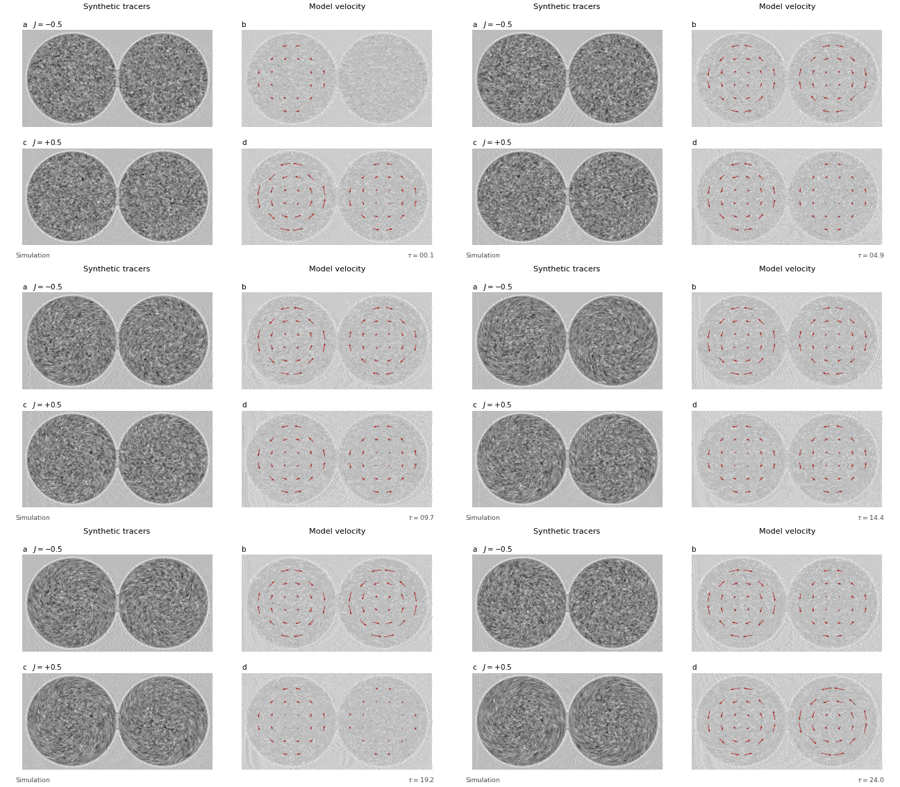
First compare the two rows in the left column, then use the arrows on the right to confirm the rotation direction in each chamber. Negative coupling makes neighbors favor opposite directions, while positive coupling favors the same direction. These preferences do not lock the vortices together like mechanical gears. Rotation strengths keep changing, and brief departures from the more common relative arrangement are possible. Interactions determine which states are favored; noise keeps the actual state fluctuating around those preferences.
A short animation shows only one finite-time realization and cannot guarantee adequate sampling of all possible states. We now turn the observation into a statistical question, comparing directional correlation and rotation strength across couplings using curves from probability integration and points from independent stochastic simulations.
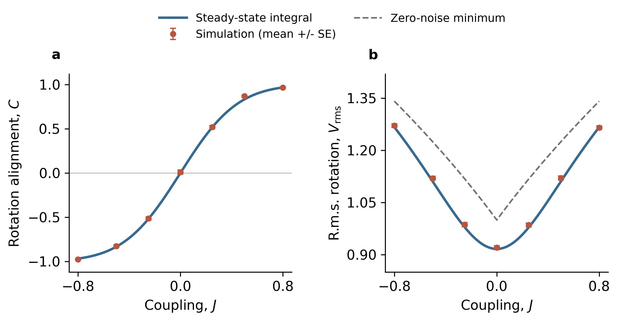
First consider the sign change in the left panel. For \(J<0\), opposite rotations lower the coupling energy and \(C<0\); for \(J>0\), rotation in the same direction is favored and \(C>0\). At \(J=0\), the chambers evolve independently, with no statistical preference for equal or opposite directions, so \(C=0\). This turns the tendencies seen in the animation into a calculable curve. However, two finite variables produce only a smooth change; the curve's passage through zero is not a thermodynamic phase transition.
Next consider the left-right symmetry of the right panel. Replacing \(J\) by \(-J\) while reversing the second vortex leaves the model energy unchanged. Preferences for equal and opposite rotation directions are exchanged, but \(V_1^2\) and \(V_2^2\) remain unchanged, as does the root-mean-square rotation strength. Measuring rotation strength alone therefore cannot distinguish the two arrangements. This returns us to the order-parameter question of Section 1 and explains why the paper measures local rotation and correlations between neighbors separately.
The right panel also retains a gray dashed curve based solely on the energy minimum. In the favored relative orientation, let both vortex amplitudes equal \(v\). Then \(H_2=(a-|J|)v^2+bv^4/2\), and minimization gives
This is the optimal amplitude when noise is neglected, not the root-mean-square value obtained from the full probability distribution. In the parameter range shown, the blue solid curve lies below the dashed curve because finite noise allows the variables to visit values away from the minima. Finding an energy minimum and calculating a statistical average in the presence of fluctuations are not the same operation. This distinction connects directly to the main argument of the lecture, but is not yet a Ginzburg test of spatial fluctuations.
Two chambers cannot undergo a genuine phase transition in the thermodynamic limit, nor can they be used to extract the critical exponents or Ginzburg number discussed here. The purpose of this small calculation is to display local preferences, interactions, and statistical fluctuations as distinct ingredients. Only after separating them is it useful to proceed to the original paper's two-lattice stochastic dynamics and parameter inference.
6.4 From Choosing Variables to Testing Approximations
The bacterial-vortex example brings the lecture's central questions together in a single model. The local quartic potential describes the values favored by an individual rotational variable, interactions determine how neighbors coordinate, and stochastic motion shows that the system does not remain permanently in the most favorable state. Once these three roles are understood, we must distinguish three levels of analysis: constructing a model, solving it approximately, and assessing the reliability of that approximation. These correspond to Landau theory, the mean-field solution used in this lecture, and the Ginzburg criterion.
Landau theory first provides a method for constructing an effective description. Rather than tracking every bacterium, we choose variables that identify the order of interest and constrain the potential using symmetry and stability. In the vortex model, equivalence of opposite rotations leads to even powers, the positive quartic term limits the rotation amplitude, and neighboring couplings organize local preferences into correlated arrangements. This modeling strategy is what the example shares with Landau theory. The appearance of a quartic polynomial does not, by itself, mean that a mean-field calculation has been performed.
The mean-field approximation specifies how we solve the model. Section 2 represented the system by a uniform background \(m_0\), determined by minimizing the free energy, without calculating the feedback of spatial fluctuations on that result. By contrast, the two-vortex program retains the joint distribution of both variables; calculating a statistical average does not make it a mean-field calculation. In the statistical figure, the gray dashed curve retains only the optimal zero-noise amplitude of the two vortices, whereas the blue solid curve includes the spread of probability at finite noise. Their difference shows what is missed by retaining only the optimal state, but the dashed curve is not itself the mean-field solution of the full lattice.
The Ginzburg criterion tests whether the neglected fluctuations can still be treated as small corrections. Fluctuations in an animation are not sufficient evidence that mean-field theory fails; what matters is their magnitude relative to the mean-field background. Returning to the spatially extended equilibrium reference model, we must also determine which positions fluctuate together. Within a region set by the correlation length \(\xi\), we then compare \(\sigma_\xi\) with \(|m_0|\). Only then do we move from observing fluctuations to the self-consistency test of Section 5.
We must also distinguish the error bars in the statistical figure from the fluctuations in the Ginzburg criterion. The error bars measure how accurately we estimate a statistical mean; \(\sigma_\xi\) measures how strongly the regionally averaged order parameter itself fluctuates. Increasing the number of independent simulations can reduce the error bars, but does not remove the system's intrinsic fluctuations. Agreement between simulation points and integration curves therefore tests the consistency of two ways of solving the same model, not the validity of mean-field theory.
Viewed in this way, the paper's quartic potential, interactions, and stochastic dynamics are no longer disconnected ingredients. They allow us, in turn, to describe competition between states, understand the emergence of order, and see the statistical structure that remains beyond the optimal state. The two-vortex example makes these distinctions concrete. Applying the Ginzburg criterion requires the further step of restoring spatial correlations and testing whether the resulting fluctuations can alter predictions built around a uniform background.
Summary
We can now return to the question posed in the introduction. Can critical behavior be calculated from a specific theory? The answer developed here has two connected parts. A simple effective free energy can yield a phase transition and critical exponents, but we must also test whether the fluctuations neglected in the calculation are sufficiently small. Obtaining an answer and establishing when it is trustworthy are two tasks within the same chain of reasoning.
Landau theory supplies a free energy that describes competition between states. We first select the order of interest, then use symmetry to determine which terms are allowed and stability to determine which nonlinear terms must be retained. This yields the simplest quartic theory. Its significance goes beyond plotting a free-energy curve: it makes the system's preference for a zero or nonzero order parameter a question that can be calculated.
The mean-field approximation used here reduces that question to finding a uniform minimum. The minimum's position gives the degree of order, its local curvature determines the susceptibility, and the equilibrium-branch free energy gives the thermodynamic changes. Mean-field critical exponents follow from this sequence. Landau theory and the mean-field approximation must therefore remain distinct: the former specifies the structure of the effective description, while the latter is our first method of solving it.
Restoring spatial dependence makes it possible to test that method. The Landau-Ginzburg free energy retains both the cost of departures from a local stable value and the cost of variations between neighboring regions. Together, they determine the correlation length. Near criticality, the potential flattens, the response grows, and correlated regions expand. Spatial fluctuations omitted by the uniform description can then become important.
The Ginzburg criterion turns the question of whether fluctuations can be neglected into a comparison of relative magnitudes. On the ordered side, it divides the variance of the order parameter averaged over a correlated region by the squared background and requires
The question is not whether fluctuations exist, but whether they are small enough to sustain an expansion about the mean-field background. For the ordinary short-range scalar quartic theory considered here, this condition generally fails sufficiently close to criticality below four dimensions. Failure of mean-field theory does not make order parameters or effective free energies meaningless. It means that we must improve the treatment of fluctuations.
Bacterial vortices provide a visible example of this argument. The quartic potential and coupling help explain rotational preferences, while the animation and statistical figure distinguish an optimal state from an average that includes fluctuations. A genuine Ginzburg test must extend that comparison to correlated regions and spatial scales. The reasoning of the lecture can therefore be summarized as
Construct the free energy with Landau theory → Find the background using a mean-field approximation → Restore spatial fluctuations → Test the approximation with the Ginzburg criterion.
When fluctuations cease to be small corrections, the next task is not to abandon the effective description, but to determine how it changes with observation scale. That is the question the renormalization group will address. The next lecture, The World of the Ising Model - From the 1D Exact Solution to the 2D Critical Point, uses a specific microscopic model to compare mean-field predictions with more exact results. After that, Block Spins and Coarse-Graining - Kadanoff's Intuitive RG Picture will turn the scale-based reasoning developed here into an explicit transformation.
References
[1] WIOLAND H, WOODHOUSE F G, DUNKEL J, GOLDSTEIN R E. Ferromagnetic and antiferromagnetic order in bacterial vortex lattices[J]. Nature Physics, 2016, 12: 341–345. DOI: https://doi.org/10.1038/nphys3607
[2] LANDAU L D. On the theory of phase transitions. I[J]. Zhurnal Eksperimental'noi i Teoreticheskoi Fiziki, 1937, 7: 19–32. https://cds.cern.ch/record/480039
[3] LANDAU L D, LIFSHITZ E M. Statistical Physics: Part 1[M]. 3rd ed. Oxford: Pergamon Press, 1980. https://www.sciencedirect.com/book/monograph/9780080230399/statistical-physics
[4] GINZBURG V L. Nobel Lecture: On superconductivity and superfluidity (what I have and have not managed to do) as well as on the “physical minimum” at the beginning of the XXI century[J]. Reviews of Modern Physics, 2004, 76(3): 981–998. DOI: https://doi.org/10.1103/RevModPhys.76.981
[5] TONG D. Statistical Field Theory[EB/OL]. University of Cambridge [2026-09-13]. https://davidtong.org/teaching/statistical-field-theory/