Mean Field Model for Homogeneous Networks
Model with Clustering Attributes
The clustering coefficient of a network is simply the ratio of triangles to triplets (both open and closed). Formally, it can be defined using the network's adjacency matrix \(G\). Assume the network is undirected and unweighted, i.e., \(G\) is symmetric, and each item is 0 or 1. For matrix \(a\), we use the symbols \(||A|| = \Sigma^N_{i=1} \Sigma^N_{j=1} a_{ij}\) and \(Tr(a) = \Sigma^N_{i=1} a_{ii}\) to indicate the trace of the matrix. The number of edges is denoted by \(||G||\). Notably, the number of triangles is \(‖G^2‖−Tr(G^2)\), and the number of triangles is \(Tr(G^3)\). The clustering coefficient of the network, defined as the ratio of triangles to triplets, is:
\[ \phi = \frac {Tr(G^3)} {||G^2|| - Tr(G^2)} \]Equations and expressions follow that involve \(SI\) edges, averages regarding infected nodes' neighbors, and the calculation of \(SSI\) triplets quantity. This section also explores neighbors linked to \(I\) nodes, culminating in a summarized expression for the \(SSI\) triplets quantity in the network.
Similarly, by introducing correlation \(C_{II}\), the expected \(ISI\) triplets are derived. Intuitively, the ratio factors or correlations measure the tendency of nodes with a particular status to become neighbors, in comparison to their random distribution in the network, impacting epidemic thresholds, final epidemic sizes, or epidemic states.
Analytical Form of SIS Model Under Pairwise-Based Approach
In the context of SIS dynamics, the system with closure at the triplet level is considered. Noting that adding the first two equations, \( [S]_s(t) + [I]_s(t) \) is constant and satisfies initial conditions \( [S]_s(0) + [I]_s(0) = N \), a conservation relation between singletons is derived as:
\[ [S]_s(t) + [I]_s(t) = N \]Consequently, the system can be simplified to four differential equations by substituting \( [S]_s (t) = N−[I]_s (t) \) into the equation for \(\dot {[S]_s}\). Moreover, conservation holds in a closed system, providing another relationship involving \( [SI]_s , [SS]_s \) and \( [II]_s \). The total number of connections can be represented by the average degree \(n\), and similarly, a conservation relationship among dyads is formulated.
Further relationships are established, allowing for further simplification of the SIS model using the aforementioned conservation relationships. A simplified system is derived, and by inserting subsequent conservation relationships into the system, an ordinary differential equation (ODE) system is obtained, which can be studied through phase plane analysis (with details available in section 4.7).
Correlation \(C_{AB} = \frac{N}{n} \frac{[AB]}{[A][B]}\) plays a vital role in understanding the dynamics of the propagation process. The pairwise model enables us to calculate correlations between different types of nodes. Several relations and equivalences are derived, implying that susceptible nodes are more likely to be connected to other susceptible nodes, while infected nodes are more likely to be connected to other infected nodes. The approximation obtained from the second (pairwise) approximation is always bounded above by the prevalence obtained from the first (single level) approximation.
Comparing Mean-Field Model (Approximation) and Master Equation Model (Exact)
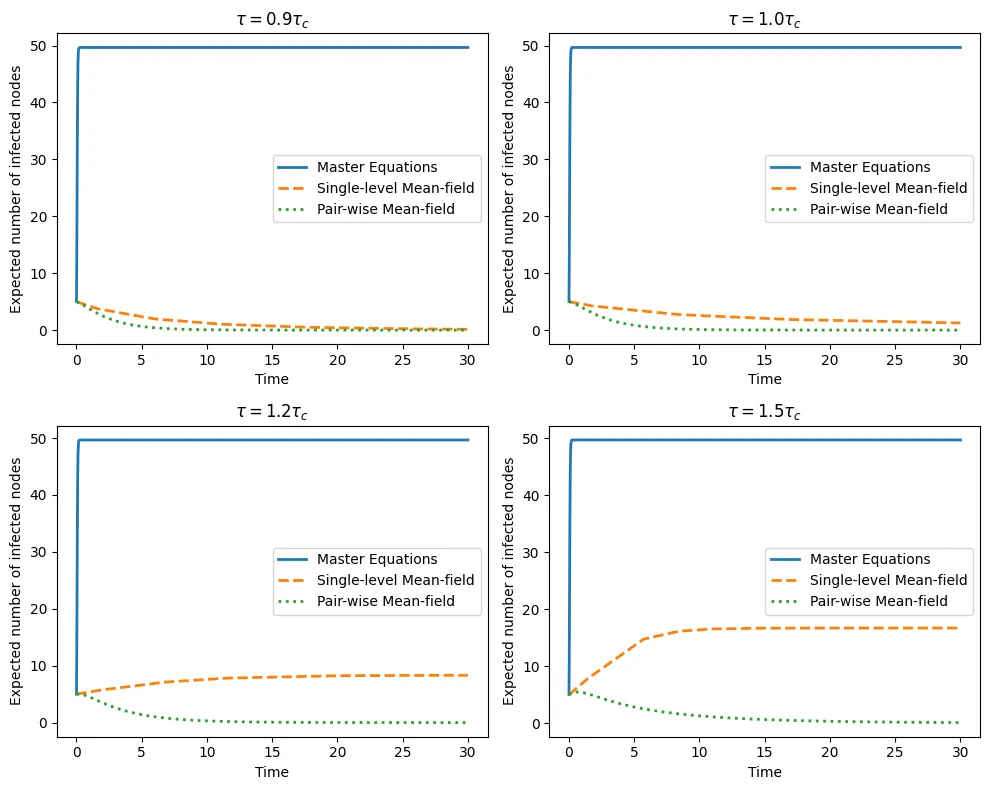
The performance of the mean-field model may depend on system parameters, i.e., the size \(N\) of the network, the values of the parameters describing epidemic dynamics, namely, the per-contact infection rate (\(\tau\)) and recovery rate (\(\gamma\)), and the network structure.
The SIS model is considered on a fully connected network of \(N\) nodes. The master equation system can be collapsed into a system with \( (N + 1) \) variables \( x_0, x_1, ..., x_N \), where \( x_k(t) \) is the probability of having \( k \) infected nodes at time \( t \). The expected number of infected nodes is \( [I](t) =\Sigma^N_{k=0} k x_k(t) \). The main comparison will be among the three functions: \( [I](t), [I]_f (t) \) and \( [I]_s(t) \).
Firstly, the influence of the parameter \(\frac{\tau}{\gamma}\), governing the dynamics of
the model, is studied. Secondly, the model is applied to two benchmark networks: ER networks and SF networks. The SIS model exhibits drastically different behaviors on these networks, and as such, they are considered separately.
This document mainly revolved around considering the SIS model on various networks and different dynamic processes. Equations, expressions, and calculations presented here seek to delve deeper into the model and apply it across different scenarios to understand its theoretical and practical implications. Though this simplification may not provide exact insights, it remains a useful approximation to glean insight into the network and its epidemiological characteristics, helping to steer research and potential interventions. Moreover, correlation and clustering attributes are crucial for analyzing the system, providing deeper insights into the spread of diseases or information across networks.
Code
We used the Python to implement the model.
                  import numpy as np
                  import matplotlib.pyplot as plt
                  from scipy.integrate import solve_ivp
                  from scipy import stats

                  # master equation system
                  def master_equations(t, Y, tau, gamma, N):
                      # Define functions for transition rates from susceptible to infected (f_TQ)
                      # and from infected to susceptible (f_QT)
                      f_TQ = lambda k: tau * k * (N - k) / N
                      f_QT = lambda k: gamma * k

                      dYdt = np.zeros(N + 1)
                      # Derivative for state with 0 infected nodes
                      dYdt[0] = f_TQ(N - 1) * Y[1] - N * f_QT(0) * Y[0]
                      # Derivative for states with 1 to N-1 infected nodes
                      dYdt[1:-1] = [(k + 1) * f_TQ(N - k - 1) * Y[k + 1] +
                                    (N - k + 1) * f_QT(k - 1) * Y[k - 1] -
                                    ((N - k) * f_QT(k) + k * f_TQ(N - k)) * Y[k] for k in range(1, N)]
                      # Derivative for state with N infected nodes
                      dYdt[-1] = f_QT(N - 1) * Y[-2] - N * f_TQ(0) * Y[-1]

                      return dYdt

                  # single-level mean-field model
                  def mean_field_single(t, y, tau, gamma, N):
                      S, I = y
                      n = N - 1
                      # Derivatives for susceptible and infected nodes
                      dSdt = gamma * I - tau * (n / N) * S * I
                      dIdt = tau * (n / N) * S * I - gamma * I
                      return [dSdt, dIdt]

                  # pair-wise mean-field model
                  def mean_field_pairwise(t, y, tau, gamma, N):
                      S, I, SI, SS, II = y
                      n = N - 1
                      # Derivatives for the numbers of susceptible nodes, infected nodes,
                      # SI edges, SS edges, and II edges respectively
                      dSdt = gamma * I - tau * SI
                      dIdt = tau * SI - gamma * I
                      dSIdt = gamma * (II - SI) + tau * ((n - 1) / n) * (SI * (SS - SI)) / S - tau * SI
                      dSSdt = 2 * gamma * SI - 2 * tau * ((n - 1) / n) * (SI * SS) / S
                      dIIdt = -2 * gamma * II + 2 * tau * ((n - 1) / n) * (SI ** 2) / S + 2 * tau * SI
                      return [dSdt, dIdt, dSIdt, dSSdt, dIIdt]

                  # Initial values
                  N = 100
                  gamma = 1
                  tau_c = gamma / (N - 1)
                  tau_values = [0.9 * tau_c, tau_c, 1.2 * tau_c, 1.5 * tau_c]
                  t_span = (0, 5)


                  I0 = 0.1 * N

                  # Initial conditions for master equations
                  # Setting the parameter lambda
                  lamb = 5
                  # Create a discrete random variable x following a Poisson distribution P(lambda)
                  x = stats.poisson(lamb)
                  # Compute the probabilities of x taking all integer values between 0 and 50 and store them in an array
                  y0_master = x.pmf(np.arange(N+1))

                  # Initial conditions for single-level mean-field model
                  y0_single = np.array([(1 - I0 / N) * N, I0])

                  # Initial conditions for pair-wise mean-field model
                  y0_pairwise = np.array([(1 - I0 / N) * N, I0, I0 * (N - I0), (N - I0) * (N - I0 - 1) / 2, I0 * (I0 - 1) / 2])

                  # Visualization
                  fig, axs = plt.subplots(2, 2, figsize=(10, 8))

                  for i, tau in enumerate(tau_values):

                      # Solve the ODE system for master equations, single-level and pair-wise mean-field models
                      sol_master = solve_ivp(master_equations, t_span, y0_master, args=(tau, gamma, N), dense_output=True)
                      I_master = np.array([np.sum([(k * sol_master.sol(t)[k]) for k in range(N + 1)]) for t in sol_master.t])

                      sol_single = solve_ivp(mean_field_single, t_span, y0_single, args=(tau, gamma, N), dense_output=True)
                      I_single = sol_single.y[1]

                      sol_pairwise = solve_ivp(mean_field_pairwise, t_span, y0_pairwise, args=(tau, gamma, N), dense_output=True)
                      I_pairwise = sol_pairwise.y[1]

                      # Plot the results
                      ax = axs[i // 2, i % 2]
                      ax.plot(sol_master.t, I_master, label='Master Equations', linewidth=2)
                      ax.plot(sol_single.t, I_single, label='Single-level Mean-field', linestyle='--', linewidth=2)
                      ax.plot(sol_pairwise.t, I_pairwise, label='Pair-wise Mean-field', linestyle=':', linewidth=2)

                      ax.set_title(f'$\\tau = {tau / tau_c:.1f} \\tau_c$')
                      ax.set_xlabel('Time')
                      ax.set_ylabel('Expected number of infected nodes')
                      ax.legend()

                  plt.tight_layout()
                  plt.show()