Percolation Model on Virus Propagation Networks
Introduction: In this chapter, we continue to update the reading notes for "Mathematics of Epidemics on Networks." Building upon the previous series, this chapter will focus on the percolation model on virus propagation networks.
Percolation Model on Virus Propagation Networks
The authors believe that percolation models and epidemiological models are essentially consistent. When considering different kinds of infectious disease models, corresponding percolation experimental designs can be found. Our observation for Erdős–Rényi random networks in Table 6.1 suggests that for the discrete time SIR model, the epidemic probability \( P \) equals the attack rate \( A \). In this section, we use percolation theory to show that this is generally true across a much wider range of networks. We will see that this result is specific to the discrete-time Markovian model. However, the tools we develop will allow us to investigate the dynamic spread of the continuous-time model in much more detail, and even make progress with non-Markovian disease processes.
Percolation is a large branch of network theory concerned with the outcome of deleting nodes or edges from networks. We will show a close relation between SIR epidemics and "bond percolation," where edges are deleted with some probability, and discuss some properties of bond percolation which are relevant to our understanding of SIR disease spread. These observations will form the basis for the remainder of the chapter. We begin with some properties of bond percolation. We then demonstrate the relationship with the discrete-time SIR model we have considered here by showing that simulating an epidemic with a given \( p \) starting from a given node is equivalent to performing bond percolation with that given \( p \) and then following edges in the remaining network from the initial node. We then use this fact to demonstrate that \( \mathcal{P} = \mathcal{A} \), and finally, we adapt the bond percolation analogy to the usual continuous-time epidemic model and our non-Markovian model.
Definition of Bond Percolation
First, the authors define the percolated network, presenting how to describe a network that has undergone the percolation process.
Given a network \( G \) and probability \( p \), we define the percolated network \( H \) to be the new network formed by taking a copy of \( G \) and deleting each edge independently with probability \( 1 − p \).
Subsequently, the authors defined what is called a connected component, an important feature of percolated networks, and a key tool for network analysis.
A set of nodes \( B \) in an undirected network forms a connected component if there is a path between any two nodes in \( B \), and no node in \( B \) has an edge to any node outside of \( B \).
After providing the two definitions, the authors further introduced the process of bond percolation. If we delete many edges in a network, it eventually breaks into multiple connected components. Typically, if \( G \) and \( p \) are large enough, then \( H \) has a single large "giant" connected component and possibly many other much smaller connected components. The precise definition of a giant component is somewhat vague for a fixed finite network, as was the definition of an epidemic. However, as the network grows larger and/or \( p \) grows, the distinction between giant components and smaller components becomes clearer.
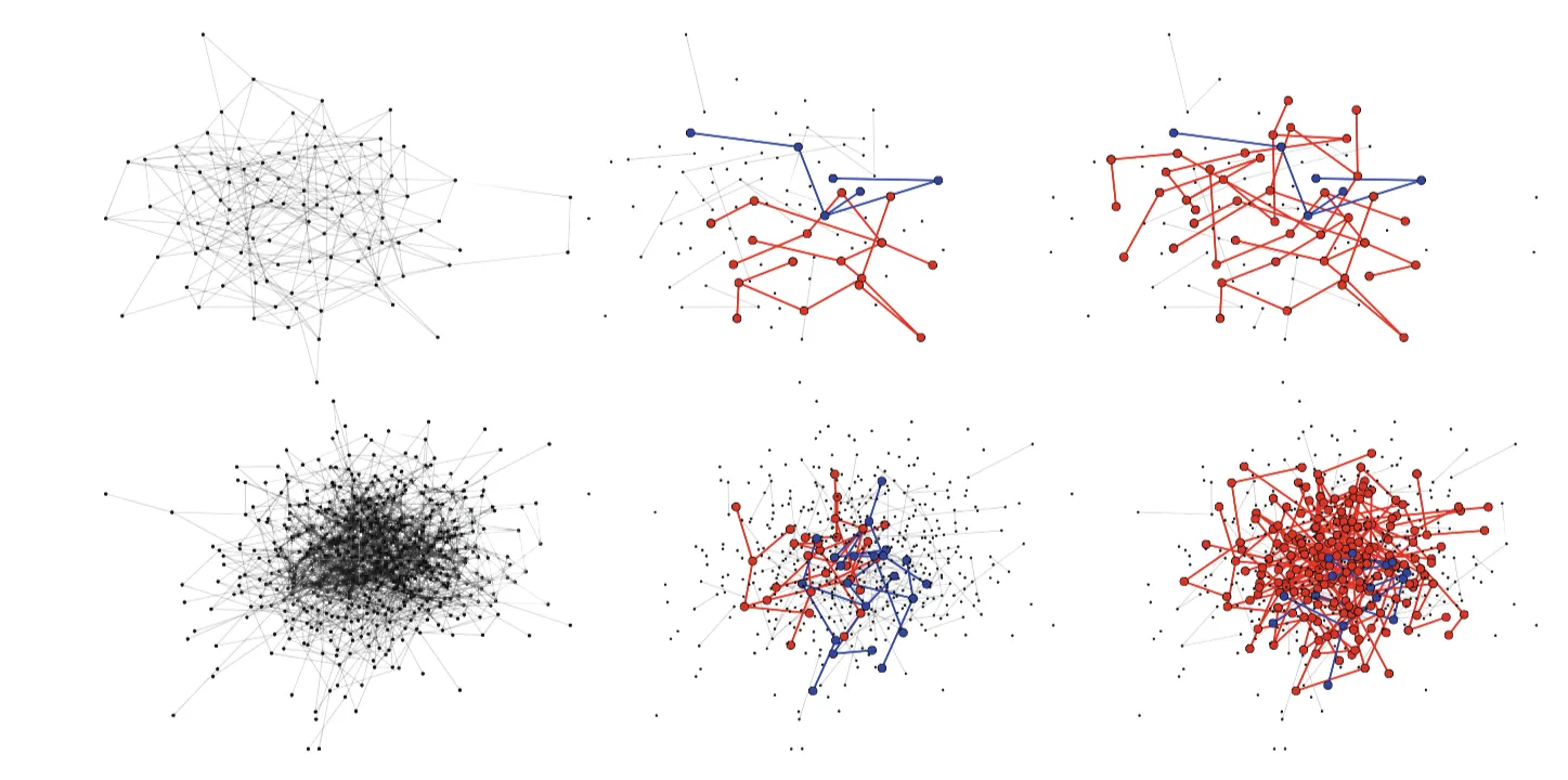
_Figure 1_ shows the result of percolation for different values of \( p \) and different network sizes in Erdős-Rényi random networks of expected degree 5. As we increase the network size for small \( p \), the largest component grows slowly and is not significantly larger than the second largest component. As \( N \rightarrow \infty \), the proportion of the nodes in the largest component goes to zero. This changes abruptly at some \( p=p_c \) (here \( p_c=0.2 \)), known as the percolation threshold. Above \( p_c \), the largest component is significantly larger than the second largest component. As \( N \rightarrow \infty \), the proportion of nodes in the largest component goes to a non-zero limit. _Figure 1_ shows that the transition becomes sharper as \( N \) increases.
The above infectious process is actually a discrete Markov percolation process, and the author has provided a pseudocode to implement this process.
          Input: Network G, index node(s) initial_infecteds, and transmission probability p.
          Output: Lists t, S, I, and R giving number in each status at each time.

          function discrete SIR epidemic(G, test transmission, parameters, initial infecteds)
              infecteds initial infectedst, S, I, R [0], [N-length(Infecteds)], [length(Infecteds)], [0]
              for u in G.nodes do
                  u.susceptible True
              for u in infecteds do
                  u.susceptible False
              while infecteds is not Empty do
                  new infecteds []
                  for u in infecteds do
                      for v in G.neighbours(u) do
                          if v.susceptible and test transmission(u, v, parameters) then
                              new infecteds.append(v)
                              v.susceptible False
                  infecteds new infecteds
                  R.append(R.last + I.last)
                  I.append(length(infecteds))
                  S.append(S.last - I.last)
                  t.append(t.last+1)
              return t, S, I, R

          function simple test transmission (u, v, [p])
              return random(0,1)< p  # Returns True with probability p.

          function basic discrete SIR epidemic (G, p, initial infecteds)
              return discrete SIR epidemic(G, simple test transmission, [p], initial infecteds)
The algorithm above is used to calculate the number of infected at each time, assuming infections last a single time step. The function `discrete_SIR_epidemic` calculates the events occurring in the outbreak. When the algorithm considers transmission from \( u \) to \( v \), it calls an auxiliary function `test transmission`. The function `basic_discrete_SIR_epidemic` implements the discrete-time Markovian model by calling `discrete_SIR_epidemic` with appropriate inputs. In this case, `simple_test_transmission` returns True with probability \( p \).
Through studying the above process, the author found the following conclusion: The proof relies on the fact that for \( N → ∞ \), after percolation in one of these networks, the giant component always occupies the same proportion. The probability of an epidemic is the probability that the initial node is in the giant component, which equals this fraction. If an epidemic occurs, the entire component is infected, so the proportion infected is also this fraction.
In addition to introducing the above discrete timestep Markov process, the author also demonstrated the continuous timestep percolation process and the spreading process that does not follow Markovian rules.
In summary, this chapter shows that the spread of the virus on the network can be regarded as a percolation process, revealing that percolation theory is a useful tool to study virus propagation on the network, and is applicable to a wide range of networks, models, and processes.
Code
We used the Python code to demonstrate the percolation process.
import networkx as nx
import numpy as np
import matplotlib.pyplot as plt
def er_random_network(N, P):
# Generate an empty undirected graph
G = nx.Graph()
# Add N nodes
G.add_nodes_from(range(N))
# Iterate through all possible edges
for i in range(N):
for j in range(i+1, N):
# Add an edge with probability P
if np.random.random() < P:
G.add_edge(i, j)
# Return the generated network
return G
def percolation_process(G, p):
# Get the number of nodes and edges in the network
N = G.number_of_nodes()
M = G.number_of_edges()
# Copy the edge set of the network for random deletion
edges = list(G.edges())
# Initialize an empty list to store the fraction of the largest connected component at each time step
fractions = []
# Initialize the time step to 0
t = 0
# Execute the loop while the network still has edges
while M > 0:
# Randomly select an edge
i = np.random.randint(M)
edge = edges[i]
# Delete the edge with probability p
if np.random.random() < p:
G.remove_edge(*edge)
edges.pop(i)
M -= 1
# Calculate the number of nodes in the network's largest connected component
largest_cc = max(nx.connected_components(G), key=len)
size = len(largest_cc)
# Calculate the fraction of the largest connected component and add it to the list
fraction = size / N
fractions.append(fraction)
# Increase the time step
t += 1
# Return the list of fractions of the largest connected component at each time step
return fractions
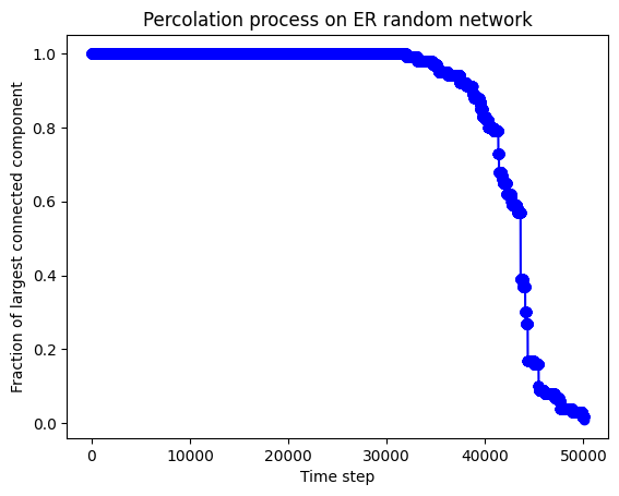
def plot_fractions(fractions):
# Get the number of time steps
T = len(fractions)
# Create an array to represent the time axis
times = np.arange(T)
# Create a figure object and a subplot object
fig, ax = plt.subplots()
# Plot a line graph on the subplot, with time on the x-axis and the fraction of the largest connected component on the y-axis
ax.plot(times, fractions, color='blue', marker='o')
# Set the title and labels of the subplot's axes
ax.set_title('Percolation process on ER random network')
ax.set_xlabel('Time step')
ax.set_ylabel('Fraction of largest connected component')
# Display the plot
plt.show()
# Generate an ER random network
G = er_random_network(100, 0.1)
# Simulate the percolation process and get a list of fractions of the largest connected component at each time step
fractions = percolation_process(G, 0.01)
# Plot a line graph to display the results of the percolation process
plot_fractions(fractions)