Top-down Dynamics Model: The Master Equation

Last updated on Oct 1, 2023 6 min read

Introduction: This article is the second in a series of reading notes on the Mathematics of epidemics on networks. Here, we primarily discuss employing the master equation to illustrate the dynamics of spread over networks. From the perspective of random processes, we introduce the master equation, often referred to as the Top-down model, which defines the state space of a system. Through this journey, we will explore Markov chains, state transition matrices, the dimensional reduction of multidimensional master equations, and more, granting us tools to accurately depict temporal and spatial changes within a system.

What the Master Equation Addresses

Consider this scenario: Disease transmission is viewed as a node transitioning between states. At any given instant, we presume that the only factors affecting the likelihood of a node altering its state are its present state and the states of its neighboring nodes. For instance, the rate at which a susceptible node gets infected is solely determined by the number of its neighbors that are infected. While neighbors can influence node transitions, the rate might also be independent of them. Specifically, the recovery rate of an infected node is not dependent on the state of any neighbor. If each node within a network of N nodes can be in one of m distinct states, then there are $m^N$ combinations of states for the entire network. For SIS, this amounts to $2^N$ states and for SIR, $3^N$ states. We term this collective set of all possible states as the state space, denoted as $\{S_1, S_2,…, S_n\}$. Ideally, we want to predict the network's state at all times.However, as the number of nodes increases, the number of equations required to describe the system also grows exponentially. This prompts us to simplify our research problem; rather than providing an equation for every state, we focus on the probability distribution of the number of states.

The primary questions addressed in this chapter can be summarized as: What's the probability of a node having a particular state at a given time? How many nodes are expected to have a certain state at a designated time?

A Basic Example

Imagine a network constituted by three nodes, with each node toggling between two possible states. This results in the network's state space comprising eight distinct states.

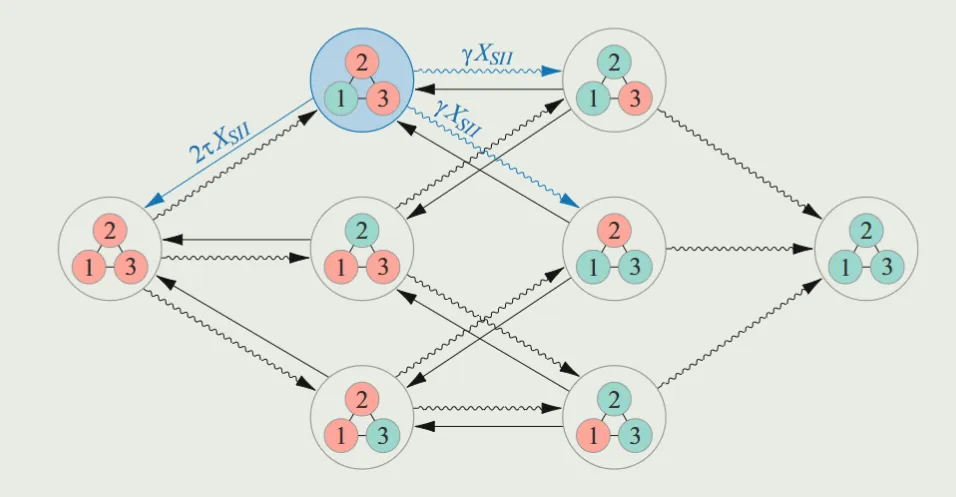
Where $τ$ represents the transmission rate and $γ$ denotes the recovery rate. Factoring in the relations between nodes, we deduce the following equations:

\begin{align} \dot{X_{SSS}} &= \gamma(X_{SSI} + X_{SIS} + X_{ISS}) \\ \dot{X_{SSI}} &= \gamma(X_{SII} + X{ISI}) - (2\tau + \gamma)X_{SSI}\\ \dot{X_{SIS}} &= \gamma(X_{SII} + X{IIS}) - (2\tau + \gamma)X_{SIS}\\ \dot{X_{ISS}} &= \gamma(X_{ISI} + X_{IIS}) - (2\tau + \gamma) X_{ISS} \\ \dot{X_{SII}} &= \gamma X_{III} + \tau(X_{SSI} + X_{SIS}) - 2(\tau + \gamma) X_{SII}\\ \dot{X_{ISI}} &= \gamma X_{III} + \tau(X_{SSI} + X_{ISS}) - 2(\tau + \gamma) X_{ISI}\\ \dot{X_{IIS}} &= \gamma X_{III} + \tau(X_{SIS} + X_{ISS}) - 2(\tau + \gamma)X_{IIS}\\ \dot{X_{III}} &= -3\gamma X_{III} + 2\tau(X_{SII}+X_{ISI} + X_{IIS}) \end{align}

**This set of equations is termed the Kolmogorov equations for the system or the master equation. Solutions to this equation provide the probability distribution of the system being in a particular state at a given moment.**

If we only need to understand the likelihood of a certain number of nodes existing in each state, the equations simplify. Instead of computing the probability of each state, we calculate the system's probability distribution based on the count of infected nodes.

\begin{align} \dot{Y_0} &= \gamma Y_1 \\ \dot{Y_1} &= 2 \gamma Y_2 - \gamma Y_1 - 2 \tau Y_1 \\ \dot{Y_2} &= 2 \tau Y_1 - 2 \gamma Y_2 - 2 \tau Y_2 + 3 \gamma Y_3 \\ \dot{Y_3} &= 2 \tau Y_2 - 3 \gamma Y_3 \end{align}

Markov Chain (Markov-chain)

Assuming the system's current state is $S_i$, $h(S_i, S_j)$ represents the rate of transition from state i to state j. A critical equation associated with the detailed balance hypothesis of Markov chains is introduced, equating the probability flowing out of state i to the probability flowing into it.

Using the aforementioned concept, we can predict the probability of the system being in a specific state at the next moment, given the information available at the current moment.

$$ P(S(t = \delta t) = S_j | S(t) = S_i) = h(S_i, S_j)\delta_t + \mathrm{o}(\delta t) $$

By integrating over the conditional probabilities, we obtain the marginal probabilities:

\[ \begin{align} X_j(t + \delta t) &= P(S(t + \delta t) = S_j) \\ &= \Sigma_{i=1}^n P(S(t + \delta t) = S_j | S(t) = S_i)P(S(t) = S_i) \\ &= \{\Sigma_{i \neq j} h(S_i, S_j) \delta t X_i(t)\} + (1 - h(S_j, S-j)\delta t) X_j(t) + \mathrm{o}(\delta t) \end{align} \]

By rearranging, we arrive at the following equation:

\[ \dot{X_j(t)} = \Sigma_{i=1}^n a_{ij}X_i(t) \]

Expressed in matrix form, this becomes:

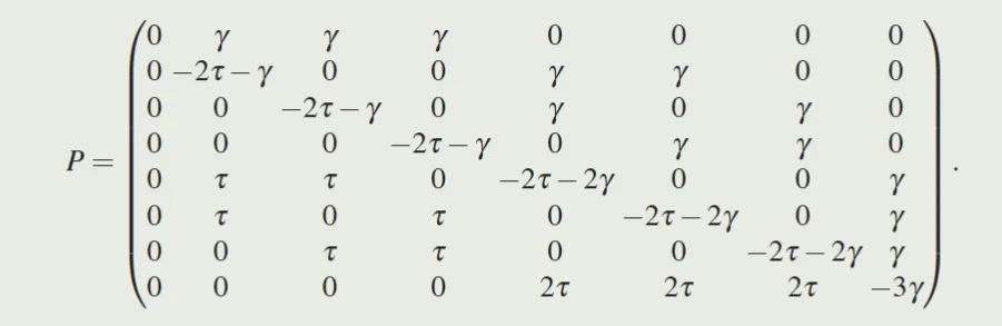
\[ \dot{X} = P \vec{X} \]

P is the state transition matrix. If there are m states and N nodes, then P is an $m^N \times m^N$ matrix. The elements of this matrix are the transition rates h we defined earlier. Next, within a given time frame, we allow only one random event to occur and provide an expression for h:

\[ f(x) = \left\{ \begin{aligned} 0, & \quad \text{if } S_{\alpha} \text{ and } S_{\beta} \text{ differ in at least two nodes} \\ f_{QT}(n_{Q1}, n_{Q2}, \ldots, n_{Qn}), & \quad \text{if } S_{\alpha} \text{ and } S_{\beta} \text{ differ at exactly node i} \\ -\Sigma_{l \neq \alpha} h(S_{\alpha}, S_l), & \quad \text{if } S_{\alpha} = S_{\beta} \end{aligned} \right. \]

State Transition Rates in the SIS Model

Now, we delve deeper into defining transition rates between different states. If the possible states of a node are {S, I}, then we introduce $S_k^j$ to depict a specific state of the system, where the superscript k denotes the number of I nodes in the network, and the subscript j represents the jth permutation of k nodes. The transition $S(k)_j \rightarrow S(k+1)_i$ signifies the transmission of a disease in a node. The rate of this transition depends on the number of neighboring nodes that are infected and is expressed as $nτ$.

The Master Equation in the SIS Model

Recall our basic example where eight equations were used to delineate the system's dynamics. We can represent these equations in matrix form: $\dot{X} = P \cdot \vec{X}$, where X denotes the system's state space. Elements of the matrix P are transition rates between states.

If we decompose matrix P, we obtain:

$$ P = \begin{pmatrix} B^0 & C^0 & 0 & 0 \\ A^1 & B^1 & C^1 & 0 \\ 0 & A^2 & B^2 & C^2 \\ 0 & 0 & A^3 & B ^ 3 \end{pmatrix} $$

From the matrix properties above, we infer:

$$ \dot{X^k} = A^kX^{k-1} + B^kX^k + C^kX^(k+1) $$

The matrix $A^k$ represents the transition from Q to T, while the matrix $C^k$ describes the transition from T to Q. These matrices depend on the structure of the network as well as the transition rates of $f_{QT}$ and $f_{TQ}$.

The element in the i-th row and j-th column of the matrix $A_k$ is represented by $A_k{i, j}$. It gives the transition rate from $S^{k−1}_j$ to $S^k_i$, which is non-zero only when there's a difference in a single node l, such that $S^{k−1}_j (l) = Q$ and $S^k_i (l) = T$. This rate depends on the number of neighbors of node l that are in state T, i.e., $A^k_{i, j} = h(S^{k−1}_j, S^k_i)$, resulting in:

\[ A^k_{i, j} = \left\{ \begin{align} 0, & \quad \text{if } S^{k-1}_j \text{ and } S^k_i \text{ differ in more than one node} \\ f_{QT}(n_T(l, S^{k-1}_j)), & \quad \text{if } S^{k-1}_j \text{ and } S^k_i \text{ differ only at node l} \end{align} \right. \]

Similarly, the entry in the i-th row and j-th column of matrix $C^k$ is represented by $C^k_{i, j}$ and gives the transition rate from $S^{k+1}_j$ to $S^k_i$.

The matrix $B^k$ is a diagonal matrix with $c_k$ rows and columns. This is because $B^k$ only indicates the transition rates of state $S^k_i \rightarrow S^k_j$. If $S_i = S_j$, the transition rate from $S^k_i$ to $S^k_j$ is zero. If $S_i \neq S_j$, then:

\[ B^k_{i, i} = -\Sigma^{c_{k+1}}_{j=1}A^{k+1}_{j, i} - \Sigma^{c_{k-1}}_{j=1}C^{k-1}_{j,i} \]

Code

Firstly, we need to establish a master equation model for an SIS model. For a fully connected network with 3 nodes, we can define the following 8 states:

All nodes are in a susceptible state: (S, S, S)
Node 1 is in an infected state, other nodes are susceptible: (I, S, S)
Node 2 is in an infected state, other nodes are susceptible: (S, I, S)
Node 3 is in an infected state, other nodes are susceptible: (S, S, I)
Nodes 1 and 2 are infected, node 3 is susceptible: (I, I, S)
Nodes 1 and 3 are infected, node 2 is susceptible: (I, S, I)
Nodes 2 and 3 are infected, node 1 is susceptible: (S, I, I)
All nodes are in an infected state: (I, I, I)

Now, we need to establish a master equation for each state. Let the infection rate be $ \beta $ and the recovery rate be $ \gamma $. For each of the aforementioned states, we can get the following master equations:

We use the Python to execute the above equations and plot the results.

                
                import numpy as np
                from scipy.integrate import odeint


                def sis_model(state, t, beta, gamma):
                    p = state
                    
                    dpdt = [
                        gamma * p[1] + gamma * p[2] + gamma * p[3] - 3 * beta * p[0],
                        beta * p[0] + gamma * p[4] - (gamma + 2 * beta) * p[1],
                        beta * p[0] + gamma * p[5] - (gamma + 2 * beta) * p[2],
                        beta * p[0] + gamma * p[6] - (gamma + 2 * beta) * p[3],
                        2 * beta * p[1] - (2 * gamma + beta) * p[4],
                        2 * beta * p[2] - (2 * gamma + beta) * p[5],
                        2 * beta * p[3] - (2 * gamma + beta) * p[6],
                        beta * p[4] + beta * p[5] + beta * p[6] - 3 * gamma * p[7]
                    ]
                    
                    return dpdt


                # Parameters
                beta = 0.5
                gamma = 0.2
                initial_state = [1, 0, 0, 0, 0, 0, 0, 0]
                t = np.linspace(0, 50, 1000)

                # Solve the systemof ODEs
                solution = odeint(sis_model, initial_state, t, args=(beta, gamma))

                # Plot the results
                import matplotlib.pyplot as plt

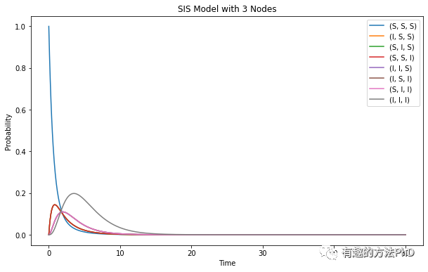
                plt.figure(figsize=(10, 6))
                plt.plot(t, solution[:, 0], label="(S, S, S)")
                plt.plot(t, solution[:, 1], label="(I, S, S)")
                plt.plot(t, solution[:, 2], label="(S, I, S)")
                plt.plot(t, solution[:, 3], label="(S, S, I)")
                plt.plot(t, solution[:, 4], label="(I, I, S)")
                plt.plot(t, solution[:, 5], label="(I, S, I)")
                plt.plot(t, solution[:, 6], label="(S, I, I)")
                plt.plot(t, solution[:, 7], label="(I, I, I)")

                plt.xlabel("Time")
                plt.ylabel("Probability")
                plt.legend()
                plt.title("SIS Model with 3 Nodes")
                plt.show()